Show code cell source Hide code cell source

# -*- coding: utf-8 -*-
# This is a report using the data from IQAASL.
# IQAASL was a project funded by the Swiss Confederation
# It produces a summary of litter survey results for a defined region.
# These charts serve as the models for the development of plagespropres.ch
# The data is gathered by volunteers.
# Please remember all copyrights apply, please give credit when applicable
# The repo is maintained by the community effective January 01, 2022
# There is ample opportunity to contribute, learn and teach
# contact dev@hammerdirt.ch

# Dies ist ein Bericht, der die Daten von IQAASL verwendet.
# IQAASL war ein von der Schweizerischen Eidgenossenschaft finanziertes Projekt.
# Es erstellt eine Zusammenfassung der Ergebnisse der Littering-Umfrage für eine bestimmte Region.
# Diese Grafiken dienten als Vorlage für die Entwicklung von plagespropres.ch.
# Die Daten werden von Freiwilligen gesammelt.
# Bitte denken Sie daran, dass alle Copyrights gelten, bitte geben Sie den Namen an, wenn zutreffend.
# Das Repo wird ab dem 01. Januar 2022 von der Community gepflegt.
# Es gibt reichlich Gelegenheit, etwas beizutragen, zu lernen und zu lehren.
# Kontakt dev@hammerdirt.ch

# Il s'agit d'un rapport utilisant les données de IQAASL.
# IQAASL était un projet financé par la Confédération suisse.
# Il produit un résumé des résultats de l'enquête sur les déchets sauvages pour une région définie.
# Ces tableaux ont servi de modèles pour le développement de plagespropres.ch
# Les données sont recueillies par des bénévoles.
# N'oubliez pas que tous les droits d'auteur s'appliquent, veuillez indiquer le crédit lorsque cela est possible.
# Le dépôt est maintenu par la communauté à partir du 1er janvier 2022.
# Il y a de nombreuses possibilités de contribuer, d'apprendre et d'enseigner.
# contact dev@hammerdirt.ch

# sys, file and nav packages:
import datetime as dt
from datetime import date, datetime, time
from babel.dates import format_date, format_datetime, format_time, get_month_names
import locale

# math packages:
import pandas as pd
import numpy as np

# charting:
import matplotlib as mpl
import matplotlib.pyplot as plt
import matplotlib.dates as mdates
from matplotlib import ticker
from matplotlib.ticker import MultipleLocator
import seaborn as sns
# from matplotlib import colors as mplcolors

# build report
import reportlab
from reportlab.lib.styles import getSampleStyleSheet, ParagraphStyle
from reportlab.lib import colors

from reportlab.platypus.flowables import Flowable
from reportlab.platypus import SimpleDocTemplate, Paragraph, Spacer, PageBreak, KeepTogether, Image
from reportlab.lib.pagesizes import A4
from reportlab.lib.units import cm
from reportlab.platypus import Table, TableStyle

# the module that has all the methods for handling the data
import resources.featuredata as featuredata
from resources.featuredata import makeAList, small_space, large_space, aSingleStyledTable, smallest_space
from resources.featuredata import caption_style, subsection_title, title_style, block_quote_style, makeBibEntry
from resources.featuredata import figureAndCaptionTable, tableAndCaption, aStyledTableWithTitleRow
from resources.featuredata import sectionParagraphs, section_title, addToDoc, makeAParagraph, bold_block
from resources.featuredata import makeAList

# home brew utitilties
import resources.sr_ut as sut

# images and display
from PIL import Image as PILImage
from IPython.display import Markdown as md
from myst_nb import glue

def convertPixelToCm(file_name: str = None):
    im = PILImage.open(file_name)
    width, height = im.size
    dpi = im.info.get("dpi", (72, 72))
    width_cm = width / dpi[0] * 2.54
    height_cm = height / dpi[1] * 2.54
    
    return width_cm, height_cm

# chart style
sns.set_style("whitegrid")

# a place to save figures and a 
# method to choose formats
save_fig_prefix = "resources/output/"

# the arguments for formatting the image
save_figure_kwargs = {
    "fname": None,
    "dpi": 300.0,
    "format": "jpeg",
    "bbox_inches": None,
    "pad_inches": 0,
    "bbox_inches": 'tight',
    "facecolor": 'auto',
    "edgecolor": 'auto',
    "backend": None,
}

## !! Begin Note book variables !!

# There are two language variants: german and english
# change both: date_lang and language
date_lang =  'de_DE.utf8'
locale.setlocale(locale.LC_ALL, date_lang)

# the date format of the survey data is defined in the module
date_format = featuredata.date_format

# the language setting use lower case: en or de
# changing the language may require changing the unit label
language = "de"
unit_label = "p/100 m"

# the standard date format is "%Y-%m-%d" if your date column is
# not in this format it will not work.
# these dates cover the duration of the IQAASL project
start_date = "2020-03-01"
end_date ="2021-05-31"
start_end = [start_date, end_date]

# the fail rate used to calculate the most common codes is
# 50% it can be changed:
fail_rate = 50

# Changing these variables produces different reports
# Call the map image for the area of interest
bassin_map = "resources/maps/rhone_city_labels.jpeg"

# the label for the aggregation of all data in the region
top = "Alle Erhebungsgebiete"

# define the feature level and components
# the feature of interest is the rhone (rhone) at the river basin (river_bassin) level.
# the label for charting is called 'name'
this_feature = {'slug':'rhone', 'name':"Erhebungsgebiet Rhône", 'level':'river_bassin'}

# the lake is in this survey area
this_bassin = "rhone"
# label for survey area
bassin_label = "Erhebungsgebiet Rhône"

# these are the smallest aggregated components
# choices are water_name_slug=lake or river, city or location at the scale of a river bassin 
# water body or lake maybe the most appropriate
this_level = 'water_name_slug'

# the doctitle is the unique name for the url of this document
doc_title = "rhone_sa"

# identify the lakes of interest for the survey area
lakes_of_interest = ["lac-leman"]

# !! End note book variables !!
## data
# Survey location details (GPS, city, land use)
dfBeaches = pd.read_csv("resources/beaches_with_land_use_rates.csv")
# set the index of the beach data to location slug
dfBeaches.set_index("slug", inplace=True)

# Survey dimensions and weights
dfDims = pd.read_csv("resources/corrected_dims.csv")

# code definitions
dxCodes = pd.read_csv("resources/codes_with_group_names_2015.csv")
dxCodes.set_index("code", inplace=True)

# columns that need to be renamed. Setting the language will automatically
# change column names, code descriptions and chart annotations
columns={"% to agg":"% agg", "% to recreation": "% recreation", "% to woods":"% woods", "% to buildings":"% buildings", "p/100m":"p/100 m"}

# !key word arguments to construct feature data
# !Note the water type allows the selection of river or lakes
# if None then the data is aggregated together. This selection
# is only valid for survey-area reports or other aggregated data
# that may have survey results from both lakes and rivers.
fd_kwargs ={
    "filename": "resources/checked_sdata_eos_2020_21.csv",
    "feature_name": this_feature['slug'], 
    "feature_level": this_feature['level'], 
    "these_features": this_feature['slug'], 
    "component": this_level, 
    "columns": columns, 
    "language": 'de', 
    "unit_label": unit_label, 
    "fail_rate": fail_rate,
    "code_data":dxCodes,
    "date_range": start_end,
    "water_type": None,    
}

fdx = featuredata.Components(**fd_kwargs)

# call the reports and languages
fdx.adjustForLanguage()
fdx.makeFeatureData()
fdx.locationSampleTotals()
fdx.makeDailyTotalSummary()
fdx.materialSummary()
fdx.mostCommon()
fdx.codeGroupSummary()

# !this is the feature data!
fd = fdx.feature_data

# !keyword args to build period data
# the period data is all the data that was collected
# during the same period from all the other locations
# not included in the feature data. For a survey area
# or river bassin these_features = feature_parent and 
# feature_level = parent_level
period_kwargs = {
    "period_data": fdx.period_data,
    "these_features": this_feature['slug'],
    "feature_level":this_feature['level'],
    "feature_parent":this_bassin,
    "parent_level": "river_bassin",
    "period_name": bassin_label,
    "unit_label": unit_label,
    "most_common": fdx.most_common.index
}
period_data = featuredata.PeriodResults(**period_kwargs)

# the rivers are considered separately
# select only the results from rivers
# this can be done by updating the fd_kwargs
fd_rivers = fd_kwargs.update({"water_type":"r"})
fdr = featuredata.Components(**fd_kwargs)
fdr.makeFeatureData()
fdr.adjustForLanguage()
fdr.makeFeatureData()
fdr.locationSampleTotals()
fdr.makeDailyTotalSummary()
fdr.materialSummary()
fdr.mostCommon()

# collects the summarized values for the feature data
# use this to generate the summary data for the survey area
# and the section for the rivers
admin_kwargs = {
    "data":fd,
    "dims_data":dfDims,
    "label": this_feature["name"],
    "feature_component": this_level,
    "date_range":start_end,
    **{"dfBeaches":dfBeaches}
}
admin_details = featuredata.AdministrativeSummary(**admin_kwargs)
admin_summary = admin_details.summaryObject()

# update the admin kwargs with river data to make the river summary
admin_kwargs.update({"data":fdr.feature_data})
admin_r_details = featuredata.AdministrativeSummary(**admin_kwargs)
admin_r_summary = admin_r_details.summaryObject()

# this defines the css rules for the note-book table displays
header_row = {'selector': 'th:nth-child(1)', 'props': f'background-color: #FFF;text-align:right;'}
even_rows = {"selector": 'tr:nth-child(even)', 'props': f'background-color: rgba(139, 69, 19, 0.08);'}
odd_rows = {'selector': 'tr:nth-child(odd)', 'props': 'background: #FFF;'}
table_font = {'selector': 'tr', 'props': 'font-size: 12px;'}
table_data = {'selector': 'td', 'props': 'padding:6px;'}
table_css_styles = [even_rows, odd_rows, table_font, header_row, table_data]

# this defines the css rules for the note-book table displays
header_row = {'selector': 'th:nth-child(1)', 'props': f'background-color: #FFF;text-align:right;'}
table_font = {'selector': 'tr', 'props': 'font-size: 12px;'}
table_data = {'selector': 'td', 'props': 'padding:6px;'}
heat_map_css_styles = [table_font, header_row, table_data]

# this is the numeric formatting for the dimensions table
dims_table_formatter = {
    "Plastik (Kg)": lambda x: featuredata.replaceDecimal(x, language),
    "Gesamtgewicht (Kg)": lambda x: featuredata.replaceDecimal(x, language),
    "Fläche (m2)": lambda x: featuredata.thousandsSeparator(int(x), language),
    "Länge (m)": lambda x: featuredata.thousandsSeparator(int(x), language),
    "Erhebungen": lambda x: featuredata.thousandsSeparator(int(x), language),
    "Objekte (St.)": lambda x: featuredata.thousandsSeparator(int(x), language)
}

# formatting for mpl charts
months = mdates.MonthLocator(interval=1)
months_fmt = mdates.DateFormatter("%b")
days = mdates.DayLocator(interval=7)

# pdf download is an option 
# the .pdf output is generated in parallel
# this is the same as if it were on the backend where we would
# have a specific api endpoint for .pdf requests. 
# reportlab is used to produce the document
# the components of the document are captured at run time
# the pdf link gives the name and location of the future doc
pdf_link = f'resources/pdfs/{this_feature["slug"]}_sa.pdf'

5. Rhône

| Download | English |

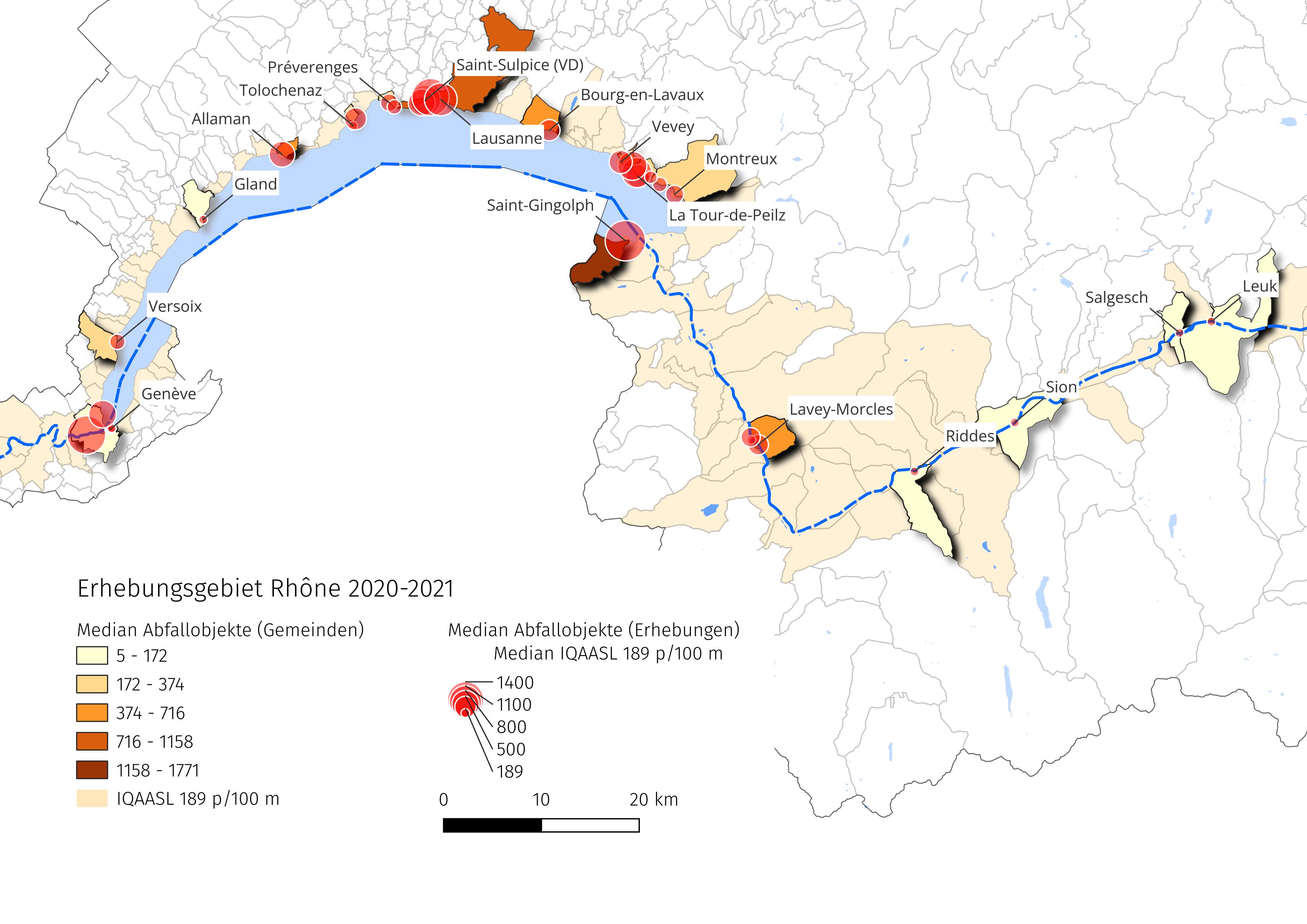
Abb. 5.1

Abbildung 5.1: Die Erhebungsorte sind für die Analyse nach Erhebungsgebiet gruppiert. Die Grösse der Markierung gibt einen Hinweis auf die Anzahl Abfallobjekte, die gefunden wurden.

5.1. Erhebungsorte und Landnutzungsprofile

Show code cell source Hide code cell source

# the admin summary can be converted into a standard text
an_admin_summary = featuredata.makeAdminSummaryStateMent(start_date, end_date, this_feature["name"], admin_summary=admin_summary)

# pdf components
new_components = [    
    small_space,
    Paragraph("Erhebungsorte", section_title), 
    small_space,
    Paragraph(an_admin_summary , featuredata.p_style),
]

# add the admin summary to the pdf
pdfcomponents = addToDoc(new_components, pdfcomponents)
# end pdf

# collect component features and land marks
# this collects the components of the feature of interest (city, lake, river)
# a comma separated string of all the componenets and a heading for each component
# type is produced
feature_components = featuredata.collectComponentLandMarks(admin_details, language=language)

# markdown output
components_markdown = "".join([f'*{x[0]}*\n\n>{x[1]}\n\n' for x in feature_components])

# put that all together:
lake_string = F"""
{an_admin_summary}

{"".join(components_markdown)}
"""

# display the string
md(lake_string)

Im Zeitraum von März 2020 bis Mai 2021 wurden im Rahmen von 106 Datenerhebungen insgesamt 28 454 Objekte entfernt und identifiziert. Die Ergebnisse des Erhebungsgebiet Rhône umfassen 32 Orte, 18 Gemeinden und eine Gesamtbevölkerung von etwa 488 138 Einwohnenden.

Seen

Lac Léman

Fliessgewässer

Rhône

Gemeinden

Allaman, Bourg-en-Lavaux, Genève, Gland, La Tour-de-Peilz, Lausanne, Lavey-Morcles, Leuk, Montreux, Préverenges, Riddes, Saint-Gingolph, Saint-Sulpice (VD), Salgesch, Sion, Tolochenaz, Versoix, Vevey

5.1.1. Kumulative Gesamtmengen nach Gewässer

Show code cell source Hide code cell source

# the basic summary of dimensional data is available in the AdministrativeSummary class
dims_table = admin_details.dimensionalSummary()
dims_table.sort_values(by=["quantity"], ascending=False, inplace=True)

# apply language settings
dims_table.rename(columns=featuredata.dims_table_columns_de, inplace=True)

# convert to kilos
dims_table["Plastik (Kg)"] = dims_table["Plastik (Kg)"]/1000

# save a copy of the dims_table for working
# formatting to pdf will turn the numerics to strings
# which eliminates any further calclations
dims_df =  dims_table.copy()

# pdf
# these columns need formatting for locale
thousands_separated = ["Fläche (m2)", "Länge (m)", "Erhebungen", "Objekte (St.)"]
replace_decimal = ["Plastik (Kg)", "Gesamtgewicht (Kg)"]

# format the dimensional summary for .pdf and add to components
dims_table[thousands_separated] = dims_table[thousands_separated].applymap(lambda x: featuredata.thousandsSeparator(int(x), language))
dims_table[replace_decimal] = dims_table[replace_decimal].applymap(lambda x: featuredata.replaceDecimal(str(round(x,2))))

# subsection title
subsection_title1 = Paragraph("Kumulative Gesamtmengen nach Gewässer", subsection_title)

# a caption for the figure
dims_table_caption = f'{this_feature["name"]}: kumulierten Gewichte  und Masse für die Gemeinden'
dims_table_captionpdf = Paragraph(dims_table_caption, style=caption_style)
# pdf table
colWidths=[3.5*cm, 3*cm, *[2.2*cm]*(len(dims_table.columns)-1)]
d_chart = aSingleStyledTable(dims_table, colWidths=colWidths)

atable = tableAndCaption(d_chart, dims_table_captionpdf, colWidths)

new_components = [
    small_space,
    subsection_title1,
    small_space,
    atable 
]
pdfcomponents = addToDoc(new_components, pdfcomponents)
# end pdf

# this formats the table through the data frame
dims_df["Plastik (Kg)"] = dims_df["Plastik (Kg)"].round(2)
dims_df["Gesamtgewicht (Kg)"] = dims_df["Gesamtgewicht (Kg)"].round(2)
dims_df[thousands_separated] = dims_df[thousands_separated].astype("int")

# set the index name to None so it doesn't show in the columns
dims_df.index.name = None
dims_df.columns.name = None

# give the figure a name
figure_name=f'{this_feature["slug"]}_dims_table'

# use the caption from the .pdf for the online figure
glue("rhone_dims_table_caption",dims_table_caption, display=False)

# apply formatting and styles to dataframe
q = dims_df.style.format(formatter=dims_table_formatter).set_table_styles(table_css_styles)

# capture the figure for display
glue(figure_name, q, display=False)

	Gesamtgewicht (Kg)	Plastik (Kg)	Fläche (m2)	Länge (m)	Erhebungen	Objekte (St.)
Erhebungsgebiet Rhône	151,31	45,97	25 986	4 911	106	28 454
Lac Léman	60,82	32,0	19 786	4 520	98	27 462
Rhône	90,48	13,97	6 200	391	8	992

Abb. 5.2

Abbildung 5.2: Erhebungsgebiet Rhône: kumulierten Gewichte und Masse für die Gemeinden

5.1.2. Landnutzungsprofil der Erhebungsorte

Das Landnutzungsprofil zeigt, welche Nutzungen innerhalb eines Radius von 1500 m um jeden Erhebungsort dominieren. Flächen werden einer von den folgenden vier Kategorien zugewiesen:

• Fläche, die von Gebäuden eingenommen wird in %

• Fläche, die dem Wald vorbehalten ist in %

• Fläche, die für Aktivitäten im Freien genutzt wird in %

• Fläche, die von der Landwirtschaft genutzt wird in %

Strassen (inkl. Wege) werden als Gesamtzahl der Strassenkilometer innerhalb eines Radius von 1500 m angegeben.

Es wird zudem angegeben, wie viele Flüsse innerhalb eines Radius von 1500 m um den Erhebungsort herum in das Gewässer münden.

Das Verhältnis der gefundenen Abfallobjekte unterscheidet sich je nach Landnutzungsprofil. Das Verhältnis gibt daher einen Hinweis auf die ökologischen und wirtschaftlichen Bedingungen um den Erhebungsort.

Für weitere Informationen siehe Landnutzungsprofil

Show code cell source Hide code cell source

# this gets all land use the data for the project
# the land use profile at 1500 m is stored with 
# location data and the survey data
land_use_kwargs = {
    "data": period_data.period_data,
    "index_column":"loc_date",
    "these_features": this_feature['slug'],
    "feature_level":this_feature['level']   
}

# the landuse profile of the project, the profile of all survey locations
project_profile = featuredata.LandUseProfile(**land_use_kwargs).byIndexColumn()

# update the kwargs for the feature data
land_use_kwargs.update({"data":fdx.feature_data})

# build the landuse profile of the feature
feature_profile = featuredata.LandUseProfile(**land_use_kwargs)

# this is the component features of the report
feature_landuse = feature_profile.featureOfInterest()

fig, axs = plt.subplots(2, 3, figsize=(9,8), sharey="row")

for i, n in enumerate(featuredata.default_land_use_columns):
    r = i%2
    c = i%3
    ax=axs[r,c]
    
    # the value of land use feature n
    # for each element of the feature
    for element in feature_landuse:
        # the land use data for a feature
        data = element[n].values
        # the name of the element
        element_name = element[feature_profile.feature_level].unique()
        # proper name for chart
        label = featuredata.river_basin_de[element_name[0]]
        # cumulative distribution        
        xs, ys = featuredata.empiricalCDF(data)
        # the plot of landuse n for this element
        sns.lineplot(x=xs, y=ys, ax=ax, label=label, color=featuredata.bassin_pallette[element_name[0]])
    
    # the value of the land use feature n for the project
    testx, testy = featuredata.empiricalCDF(project_profile[n].values)
    sns.lineplot(x=testx, y=testy, ax=ax, label=top, color="magenta")
    
    # get the median landuse for the feature
    the_median = np.median(data)
    
    # plot the median and drop horizontal and vertical lines
    ax.scatter([the_median], 0.5, color="red",s=40, linewidth=1, zorder=100, label="Median")
    ax.vlines(x=the_median, ymin=0, ymax=0.5, color="red", linewidth=1)
    ax.hlines(xmax=the_median, xmin=0, y=0.5, color="red", linewidth=1)
    
    if i <= 3:
        if c == 0:            
            ax.yaxis.set_major_locator(MultipleLocator(.1))
        ax.xaxis.set_major_formatter(ticker.PercentFormatter(1.0, 0, "%"))        
    else:
        pass      
    
    handles, labels = ax.get_legend_handles_labels()
    ax.get_legend().remove()    
    ax.set_title(featuredata.luse_de[n], loc='left')
    
# filename and figure tag
figure_name = "rhone_survey_area_landuse"
land_use_file_name = f'{save_fig_prefix}{figure_name}.jpeg'
save_figure_kwargs.update({"fname":land_use_file_name})
    
plt.subplots_adjust(top=.91, hspace=.4)
plt.suptitle("Landnutzung im Umkries von 1 500 m um den Erhebungsort", ha="center", y=1, fontsize=16)
fig.legend(handles, labels, bbox_to_anchor=(.5,.5), loc="upper center", ncol=3)

plt.tight_layout()
plt.subplots_adjust(top=.91, hspace=.4)

# save figure
plt.savefig(**save_figure_kwargs)

# capture the output
figure_caption = "Landnutzungsprofil der Erhebungsorte. Verteilung der Erhebungen in Bezug auf die Landnutzung."
glue(figure_name, fig, display=False)
glue(f"{this_feature['slug']}_land_use_caption", figure_caption, display=False)

plt.close()

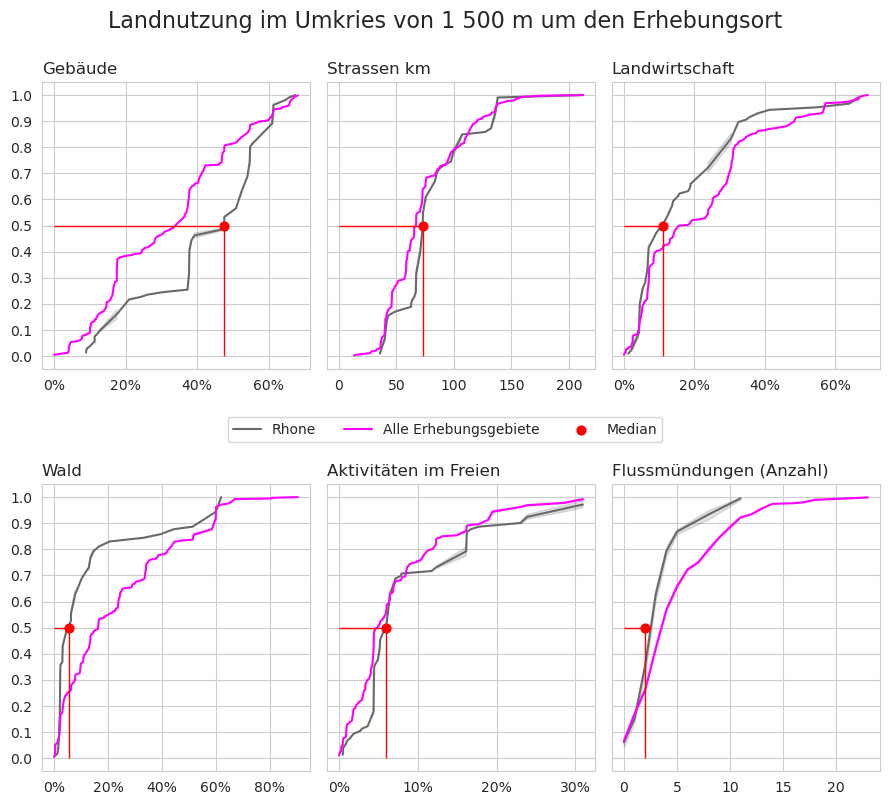
Abb. 5.3

Abbildung 5.3: Landnutzungsprofil der Erhebungsorte. Verteilung der Erhebungen in Bezug auf die Landnutzung.

5.1.3. Verteilung der Erhebungsergebnisse

Show code cell source Hide code cell source

# pdf
o_w, o_h = convertPixelToCm(land_use_file_name)
f3cap = Paragraph(figure_caption, caption_style)
figure_kwargs = {
    "image_file":land_use_file_name,
    "caption": f3cap, 
    "original_width":o_w,
    "original_height":o_h,
    "desired_width": 14,
    "caption_height":1,
    "hAlign": "CENTER",
}

f3 = figureAndCaptionTable(**figure_kwargs)

new_components = [
    small_space,
    f3
]

pdfcomponents = addToDoc(new_components, pdfcomponents)
# end pdf

# the sample totals of all other locations than the feature data
dx = period_data.parentSampleTotals(parent=False)

# get the monthly or quarterly results for the feature
rsmp = fdx.sample_totals.set_index("date")
resample_plot, rate = featuredata.quarterlyOrMonthlyValues(rsmp, this_feature["name"], vals=unit_label)

fig, axs = plt.subplots(1,2, figsize=(10,5))

ax = axs[0]

# feature surveys
sns.scatterplot(data=dx, x="date", y=unit_label, label=top, color="black", alpha=0.4,  ax=ax)
# all other surveys
sns.scatterplot(data=fdx.sample_totals, x="date", y=unit_label, label=this_feature["name"], color="red", s=34, ec="white", ax=ax)
# monthly or quaterly plot
sns.lineplot(data=resample_plot, x=resample_plot.index, y=resample_plot, label=F"{this_feature['name']}: monatlicher Medianwert", color="magenta", ax=ax)

ax.set_ylabel(unit_label, **featuredata.xlab_k14)

ax.set_xlabel("")
ax.xaxis.set_minor_locator(days)
ax.xaxis.set_major_formatter(months_fmt)
ax.set_ylim(-50, 2000)

ax.legend()

# the cumlative distributions:
axtwo = axs[1]

# the feature of interest
feature_ecd = featuredata.ecdfOfAColumn(fdx.sample_totals, unit_label)    
sns.lineplot(x=feature_ecd["x"], y=feature_ecd["y"], color="darkblue", ax=axtwo, label=this_feature["name"])

# the other features
other_features = featuredata.ecdfOfAColumn(dx, unit_label)
sns.lineplot(x=other_features["x"], y=other_features["y"], color="magenta", label=top, linewidth=1, ax=axtwo)

axtwo.set_xlabel(unit_label, **featuredata.xlab_k14)
axtwo.set_ylabel("Verhältnis der Erhebungen", **featuredata.xlab_k14)
axtwo.set_xlim(0, 3000)
axtwo.legend(bbox_to_anchor=(.4,.5), loc="upper left")
axtwo.xaxis.set_major_locator(MultipleLocator(500))
axtwo.xaxis.set_minor_locator(MultipleLocator(100))
axtwo.yaxis.set_major_locator(MultipleLocator(.1))
axtwo.grid(which="minor", visible=True, axis="x", linestyle="--", linewidth=1)

plt.tight_layout()

figure_name = f"{this_feature['slug']}_sample_totals"
sample_totals_file_name = f'{save_fig_prefix}{figure_name}.jpeg'
save_figure_kwargs.update({"fname":sample_totals_file_name})
plt.savefig(**save_figure_kwargs)

# figure caption
sample_total_notes = [
    f'Links: {this_feature["name"]}, {featuredata.dateToYearAndMonth(datetime.strptime(start_date, date_format), lang=date_lang)} ',
    f'bis {featuredata.dateToYearAndMonth(datetime.strptime(end_date, date_format), lang=date_lang)}, n = {admin_summary["loc_date"]}. ',
    f'Rechts: empirische Verteilungsfunktion der Erhebungsergebnisse {this_feature["name"]}.'
]

sample_total_notes = ''.join(sample_total_notes)

glue(f'{this_feature["slug"]}_sample_total_notes', sample_total_notes, display=False)
glue("rhone_sample_totals", fig, display=False)
plt.close()

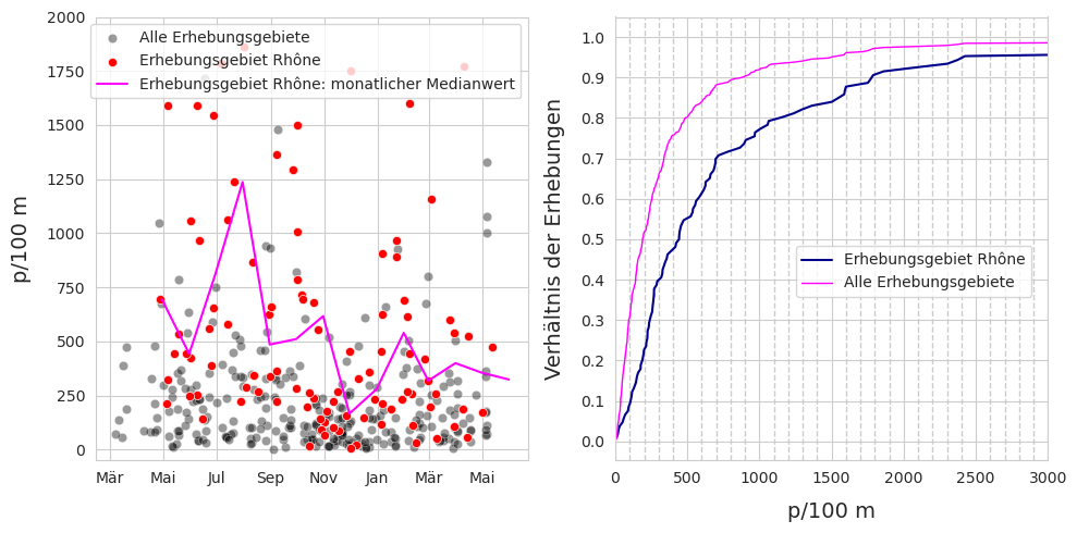
Abb. 5.4

Abbildung 5.4: Links: Erhebungsgebiet Rhône, März 2020 bis Mai 2021, n = 106. Rechts: empirische Verteilungsfunktion der Erhebungsergebnisse Erhebungsgebiet Rhône.

5.1.4. Zusammengefasste Daten und Materialarten

Show code cell source Hide code cell source

csx = fdx.sample_summary.copy()


combined_summary =[(x, featuredata.thousandsSeparator(int(csx[x]), language)) for x in csx.index]

# the materials table
fd_mat_totals = fdx.material_summary.copy()
fd_mat_totals = featuredata.fmtPctOfTotal(fd_mat_totals, around=0)

# applly new column names for printing
cols_to_use = {"material":"Material","quantity":"Objekte (St.)", "% of total":"Anteil"}
fd_mat_t = fd_mat_totals[cols_to_use.keys()].values
fd_mat_t = [(x[0], featuredata.thousandsSeparator(int(x[1]), language), x[2]) for x in fd_mat_t]

# make tables
fig, axs = plt.subplots(1,2)

# summary table
# names for the table columns
a_col = [this_feature["name"], "Total"]

axone = axs[0]
featuredata.hide_spines_ticks_grids(axone)

table_two = sut.make_a_table(axone, combined_summary,  colLabels=a_col, colWidths=[.75,.25],  bbox=[0,0,1,1], **{"loc":"lower center"})
table_two.get_celld()[(0,0)].get_text().set_text(" ")
table_two.set_fontsize(12)

# material table
axtwo = axs[1]
axtwo.set_xlabel(" ")
featuredata.hide_spines_ticks_grids(axtwo)

table_three = sut.make_a_table(axtwo, fd_mat_t,  colLabels=list(cols_to_use.values()), colWidths=[.4, .4,.2],  bbox=[0,0,1,1], **{"loc":"lower center"})
table_three.get_celld()[(0,0)].get_text().set_text(" ")
table_three.set_fontsize(12)
plt.tight_layout()
plt.subplots_adjust(wspace=0.2)

# figure caption
summary_of_survey_totals = [
    f'Zusammenfassung der Daten aller Erhebungen am {this_feature["name"]}. ',
    f'Gefunden Materialarten am {this_feature["name"]} in Stückzahlen und ',
    f'als prozentuale Anteile (stückzahlbezogen).'
]

summary_of_survey_totals = ''.join(summary_of_survey_totals)
glue(f'{this_feature["slug"]}_sample_summaries_caption', summary_of_survey_totals, display=False)

figure_name = f'{this_feature["slug"]}_sample_summaries'
sample_summaries_file_name = f'{save_fig_prefix}{figure_name}.jpeg'
save_figure_kwargs.update({"fname":sample_summaries_file_name})

plt.savefig(**save_figure_kwargs)
glue('rhone_survey_area_sample_material_tables', fig, display=False)
plt.close()

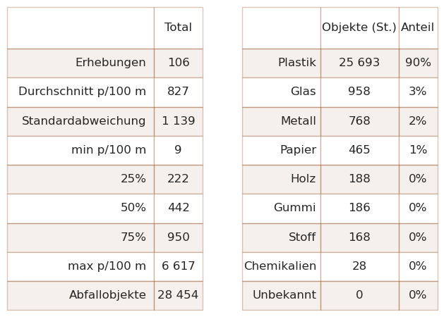
Abb. 5.5

Abbildung 5.5: Zusammenfassung der Daten aller Erhebungen am Erhebungsgebiet Rhône. Gefunden Materialarten am Erhebungsgebiet Rhône in Stückzahlen und als prozentuale Anteile (stückzahlbezogen).

5.2. Die am häufigsten gefundenen Objekte

Die am häufigsten gefundenen Objekte sind die zehn mengenmässig am meisten vorkommenden Objekte und/oder Objekte, die in mindestens 50 % aller Datenerhebungen identifiziert wurden (Häufigkeitsrate)

Show code cell source Hide code cell source

# add summary tables to pdf
sample_summary_subsection = Paragraph("Verteilung der Erhebungsergebnisse", subsection_title)

sample_total_notes_pdf = [
    f'<b>Links:</b> {this_feature["name"]}, {featuredata.dateToYearAndMonth(datetime.strptime(start_date, date_format), lang=date_lang)} ',
    f'bis {featuredata.dateToYearAndMonth(datetime.strptime(end_date, date_format), lang=date_lang)}, n = {admin_summary["loc_date"]}. ',
    f'<b>Rechts:</b> empirische Verteilungsfunktion der Erhebungsergebnisse {this_feature["name"]}.'
]
s_totals_caption = makeAParagraph(sample_total_notes_pdf, style=caption_style)

samp_mat_subsection = Paragraph("Zusammengefasste Daten und Materialarten", style=subsection_title)
samp_material_caption = Paragraph(summary_of_survey_totals, style=caption_style)

o_w, o_h = convertPixelToCm(sample_totals_file_name)

figure_kwargs = {
    "image_file":sample_totals_file_name,
    "caption": s_totals_caption, 
    "original_width":o_w,
    "original_height":o_h,
    "desired_width": 15,
    "caption_height":1,
    "hAlign": "CENTER",
}

f4 = figureAndCaptionTable(**figure_kwargs)

o_w, o_h = convertPixelToCm(sample_summaries_file_name)

figure_kwargs = {
    "image_file":sample_summaries_file_name,
    "caption": samp_material_caption, 
    "original_width":o_w,
    "original_height":o_h,
    "desired_width": 11,
    "caption_height":1,
    "hAlign": "CENTER",
}

f5 = figureAndCaptionTable(**figure_kwargs)


new_components = [
    PageBreak(),
    sample_summary_subsection,
    small_space,
    f4,
    small_space,
    samp_mat_subsection,
    small_space,
    f5,
    PageBreak()
]

pdfcomponents = addToDoc(new_components, pdfcomponents)

# the most common objects results
most_common_display = fdx.most_common

# language appropriate columns
cols_to_use = featuredata.most_common_objects_table_de
cols_to_use.update({unit_label:unit_label})

# data for display
most_common_display.rename(columns=cols_to_use, inplace=True)
most_common_display = most_common_display[cols_to_use.values()].copy()
most_common_display = most_common_display.set_index("Objekte", drop=True)

# .pdf output
data = most_common_display.copy()
data["Anteil"] = data["Anteil"].map(lambda x: f"{int(x)}%")
data['Objekte (St.)'] = data['Objekte (St.)'].map(lambda x:featuredata.thousandsSeparator(x, language))
data['Häufigkeitsrate'] = data['Häufigkeitsrate'].map(lambda x: f"{x}%")
data[unit_label] = data[unit_label].map(lambda x: featuredata.replaceDecimal(round(x,1)))

# make caption
# get percent of total to make the caption string
m_common_percent_of_total = fdx.most_common['Objekte (St.)'].sum()/fdx.code_summary['quantity'].sum()

mc_caption_string = [
    f'Häufigste Objekte im {this_feature["name"]}: ',
    'd. h. Objekte mit einer Häufigkeitsrate von mindestens 50% und/oder ',
    f'Top Ten nach Anzahl. Zusammengenommen machen die häufigsten Objekte {int(m_common_percent_of_total*100)}% ',
    f'aller gefundenen Objekte aus. Anmerkung: {unit_label} = Medianwert der Erhebung.'
]

mc_caption_string = "".join(mc_caption_string)

colwidths = [4.5*cm, 2.2*cm, 2*cm, 2.8*cm, 2*cm]

mc_caption_string = "".join(mc_caption_string)
d_chart = aSingleStyledTable(data, colWidths=colwidths)
d_capt = featuredata.makeAParagraph(mc_caption_string, style=caption_style)
mc_table = tableAndCaption(d_chart, d_capt, colwidths)

most_common_display.index.name = None
most_common_display.columns.name = None

# set pandas display
aformatter = {
    "Anteil":lambda x: f"{int(x)}%",
    f"{unit_label}": lambda x: featuredata.replaceDecimal(x, language),
    "Häufigkeitsrate": lambda x: f"{int(x)}%",   
    "Objekte (St.)": lambda x: featuredata.thousandsSeparator(int(x), language)
}

mcd = most_common_display.style.format(aformatter).set_table_styles(table_css_styles)
glue('rhone_most_common_caption', mc_caption_string, display=False)
glue('rhone_most_common_tables', mcd, display=False)

	Objekte (St.)	Anteil	Häufigkeitsrate	p/100 m
Fragmentierte Kunststoffe	4 220	14%	93%	48,0
Expandiertes Polystyrol	3 589	12%	80%	17,5
Zigarettenfilter	3 169	11%	90%	41,5
Snack-Verpackungen	1 737	6%	92%	19,0
Industriepellets (Nurdles)	1 387	4%	43%	0,0
Industriefolie (Kunststoff)	1 180	4%	76%	9,0
Wattestäbchen/Tupfer	1 112	3%	75%	10,5
Schaumstoffverpackungen/Isolierung	1 112	3%	71%	7,0
Styropor < 5mm	718	2%	28%	0,0
Kunststoff-Bauabfälle	614	2%	65%	5,5
Getränkeflaschen aus Glas, Glasfragmente	554	1%	54%	2,0
Getränke-Deckel, Getränkeverschluss	425	1%	51%	1,0
Ringe von Plastikflaschen/Behältern	362	1%	68%	4,0
Kronkorken, Lasche von Dose/Ausfreisslachen	350	1%	67%	3,0
Schrotflintenpatronen	347	1%	50%	0,5
Tabak; Kunststoffverpackungen, Behälter	296	1%	51%	1,0
Strohhalme und Rührstäbchen	278	0%	67%	3,5
unidentifizierte Deckel	263	0%	54%	2,0
Schleckstengel, Stengel von Lutscher	238	0%	62%	2,5
Einwegartikel; Tassen/Becher & Deckel	201	0%	55%	2,0
Spielzeug und Partyartikel	194	0%	60%	2,0
Verpackungen aus Aluminiumfolie	178	0%	52%	1,0
Medizin; Behälter/Röhrchen/Verpackungen	177	0%	57%	2,0

Abb. 5.6

Abbildung 5.6: Häufigste Objekte im Erhebungsgebiet Rhône: d. h. Objekte mit einer Häufigkeitsrate von mindestens 50% und/oder Top Ten nach Anzahl. Zusammengenommen machen die häufigsten Objekte 79% aller gefundenen Objekte aus. Anmerkung: p/100 m = Medianwert der Erhebung.

5.2.1. Die am häufigsten gefundenen Objekte nach Gewässer

Show code cell source Hide code cell source

# add new section to pdf
mc_section_title = Paragraph("Die am häufigsten gefundenen Objekte", section_title)
para_g = "Die am häufigsten gefundenen Objekte sind die zehn mengenmässig am meisten vorkommenden Objekte und/oder Objekte, die in mindestens 50 % aller Datenerhebungen identifiziert wurden (Häufigkeitsrate)"
mc_section_para = Paragraph(para_g, featuredata.p_style)

new_components = [
    KeepTogether([
        mc_section_title,
        small_space,
        mc_section_para
    ]),
    small_space,
    mc_table,
       
]
pdfcomponents = addToDoc(new_components, pdfcomponents)

mc_heat_map_caption = f'Median {unit_label} der häufigsten Objekte am {this_feature["name"]}.'

# calling componentsMostCommon gets the results for the most common codes
# at the component level
components = fdx.componentMostCommonPcsM()

# map to proper names for features
feature_names = admin_details.makeFeatureNameMap()

# pivot that and quash the hierarchal column index that is created when the table is pivoted
mc_comp = components[["item", unit_label, this_level]].pivot(columns=this_level, index="item")
mc_comp.columns = mc_comp.columns.get_level_values(1)

# insert the proper columns names for display
proper_column_names = {x : feature_names.loc[x, 'water_name'] for x in mc_comp.columns}
mc_comp.rename(columns = proper_column_names, inplace=True)

# the aggregated total of the feature is taken from the most common objects table
mc_feature = fdx.most_common[unit_label]
mc_feature = featuredata.changeSeriesIndexLabels(mc_feature, {x:fdx.dMap.loc[x] for x in mc_feature.index})

# the aggregated totals of all the period data
mc_period = period_data.parentMostCommon(parent=False)
mc_period = featuredata.changeSeriesIndexLabels(mc_period, {x:fdx.dMap.loc[x] for x in mc_period.index})

# add the feature, bassin_label and period results to the components table
mc_comp[this_feature["name"]]= mc_feature
mc_comp[top] = mc_period

caption_prefix =  f'Median {unit_label} der häufigsten Objekte am '
col_widths=[4.5*cm, *[1*cm]*(len(mc_comp.columns))]
mc_heatmap_title = Paragraph("Die am häufigsten gefundenen Objekte nach Gewässer", subsection_title)
tables = featuredata.splitTableWidth(mc_comp, gradient=True, caption_prefix=caption_prefix, caption=mc_heat_map_caption,
                    this_feature=this_feature["name"], vertical_header=True, colWidths=col_widths)

# identify the tables variable as either a list or a Flowable:
if isinstance(tables, (list, np.ndarray)):
    grouped_pdf_components = [*tables]
else:
    grouped_pdf_components = [tables]
    

new_components = [
    small_space,
    mc_heatmap_title,
    small_space,
    *grouped_pdf_components
]

pdfcomponents = addToDoc(new_components, pdfcomponents)

# notebook display style
aformatter = {x: featuredata.replaceDecimal for x in mc_comp.columns}

mcd = mc_comp.style.format(aformatter).set_table_styles(heat_map_css_styles)
mcd = mcd.background_gradient(axis=None, vmin=mc_comp.min().min(), vmax=mc_comp.max().max(), cmap="YlOrBr")

# remove the index name and column name labels
mcd.index.name = None
mcd.columns.name = None

# rotate the text on the header row
# the .applymap_index method in the
# df.styler module is used for this
mcd = mcd.applymap_index(featuredata.rotateText, axis=1)

# display markdown html
glue(f'{this_feature["slug"]}_mc_heat_map_caption', mc_heat_map_caption, display=False)

glue(f'{this_feature["slug"]}_most_common_heat_map', mcd, display=False)

	Lac Léman	Rhône	Erhebungsgebiet Rhône	Alle Erhebungsgebiete
Getränkeflaschen aus Glas, Glasfragmente	3,0	0,0	2,0	3,0
Einwegartikel; Tassen/Becher & Deckel	2,0	0,0	2,0	0,0
Expandiertes Polystyrol	26,0	0,0	17,5	5,0
Fragmentierte Kunststoffe	61,5	0,5	48,0	18,0
Getränke-Deckel, Getränkeverschluss	2,0	0,0	1,0	0,0
Industriefolie (Kunststoff)	9,0	18,0	9,0	5,0
Industriepellets (Nurdles)	0,0	0,0	0,0	0,0
Kronkorken, Lasche von Dose/Ausfreisslachen	3,0	0,0	3,0	1,0
Kunststoff-Bauabfälle	5,5	3,5	5,5	1,0
Medizin; Behälter/Röhrchen/Verpackungen	2,0	0,0	2,0	0,0
Ringe von Plastikflaschen/Behältern	4,0	0,0	4,0	0,0
Schaumstoffverpackungen/Isolierung	10,0	0,0	7,0	1,0
Schleckstengel, Stengel von Lutscher	3,0	0,0	2,5	0,0
Schrotflintenpatronen	1,0	0,0	0,5	0,0
Snack-Verpackungen	21,5	1,0	19,0	9,0
Spielzeug und Partyartikel	2,5	0,0	2,0	0,0
Strohhalme und Rührstäbchen	4,0	0,0	3,5	0,0
Styropor < 5mm	0,0	0,0	0,0	0,0
Tabak; Kunststoffverpackungen, Behälter	2,0	0,0	1,0	0,0
Verpackungen aus Aluminiumfolie	2,0	0,0	1,0	0,0
Wattestäbchen/Tupfer	12,0	0,0	10,5	1,0
Zigarettenfilter	47,0	0,0	41,5	20,0
unidentifizierte Deckel	2,0	0,0	2,0	0,0

Abb. 5.7

Abbildung 5.7: Median p/100 m der häufigsten Objekte am Erhebungsgebiet Rhône.

5.2.2. Die am häufigsten gefundenen Objekte im monatlichen Durchschnitt

Show code cell source Hide code cell source

# collect the survey results of the most common objects
# and aggregate code with groupname for each sample
# use the index from the most common codes to select from the feature data
# the aggregation method and the columns to keep
agg_pcs_quantity = {unit_label:"sum", "quantity":"sum"}
groups = ["loc_date","date","code", "groupname"]
# make the range for one calendar year
start_date = "2020-04-01"
end_date = "2021-03-31"
# aggregate
m_common_m = fd[(fd.code.isin(fdx.most_common.index))].groupby(groups, as_index=False).agg(agg_pcs_quantity)
# set the index to the date column and sort values within the date rage
m_common_m.set_index("date", inplace=True)
m_common_m = m_common_m.sort_index().loc[start_date:end_date]

# set the order of the chart, group the codes by groupname columns and collect the respective object codes
an_order = m_common_m.groupby(["code","groupname"], as_index=False).quantity.sum().sort_values(by="groupname")["code"].values

# use the order array and resample each code for the monthly value
# store in a dict
mgr = {}
for a_code in an_order:
    # resample by month
    a_cell = m_common_m[(m_common_m.code==a_code)][unit_label].resample("M").mean().fillna(0)
    a_cell = round(a_cell, 1)
    this_group = {a_code:a_cell}
    mgr.update(this_group)

# make df form dict and collect the abbreviated month name set that to index
by_month = pd.DataFrame.from_dict(mgr)
by_month["month"] = by_month.index.map(lambda x: get_month_names('abbreviated', locale=date_lang)[x.month])
by_month.set_index('month', drop=True, inplace=True)

# transpose to get months on the columns and set index to the object description
by_month = by_month.T
by_month["Objekt"] = by_month.index.map(lambda x: fdx.dMap.loc[x])
by_month.set_index("Objekt", drop=True, inplace=True)

# pdf components
# gradient background for .pdf table
monthly_heat_map_gradient = featuredata.colorGradientTable(by_month)

# subsection title and figure caption
mc_monthly_title = Paragraph("Die am häufigsten gefundenen Objekte im monatlichen Durchschnitt", subsection_title)
monthly_data_caption = f'{this_feature["name"]}, monatliche Durchschnittsergebnisse p/100 m'
figure_caption = Paragraph(monthly_data_caption, caption_style)

# make pdf table
col_widths = [4.5*cm, *[1*cm]*(len(mc_comp.columns))]

d_chart = aSingleStyledTable(by_month, vertical_header=True, gradient=True, colWidths=col_widths)
d_capt = featuredata.makeAParagraph(monthly_data_caption, style=caption_style)
mc_table = tableAndCaption(d_chart, d_capt, colwidths)
new_components = [
    KeepTogether([
        featuredata.large_space,
        mc_monthly_title,
        featuredata.large_space,
        mc_table
    ])
]

pdfcomponents = addToDoc(new_components, pdfcomponents)

# remove the index names for .html display
by_month.index.name = None
by_month.columns.name = None

aformatter = {x: featuredata.replaceDecimal for x in by_month.columns}

mcdm = by_month.style.format(aformatter).set_table_styles(heat_map_css_styles).background_gradient(axis=None, cmap="YlOrBr", vmin=by_month.min().min(), vmax=by_month.max().max())
glue("rhone_monthly_results_caption", monthly_data_caption, display=False)
glue("rhone_monthly_results", mcdm, display=False)

	Apr.	Mai	Juni	Juli	Aug.	Sept.	Okt.	Nov.	Dez.	Jan.	Feb.	März
Medizin; Behälter/Röhrchen/Verpackungen	5,0	4,3	13,8	6,3	6,4	4,2	7,1	4,7	9,1	4,0	2,0	8,6
Wattestäbchen/Tupfer	7,0	31,9	56,8	80,3	38,8	23,0	26,2	11,4	36,0	26,4	14,6	33,6
Strohhalme und Rührstäbchen	16,0	9,7	13,8	16,6	6,0	8,7	5,1	2,3	3,8	8,5	0,8	13,9
Einwegartikel; Tassen/Becher & Deckel	9,0	6,6	3,4	12,7	5,1	3,8	4,2	1,5	3,6	6,7	3,4	11,9
Schleckstengel, Stengel von Lutscher	9,0	8,1	10,6	16,3	9,5	11,2	3,8	1,3	10,9	5,8	2,3	6,6
Ringe von Plastikflaschen/Behältern	5,0	5,9	12,8	18,1	10,2	5,5	10,1	5,3	5,8	8,2	11,0	22,0
Snack-Verpackungen	91,0	20,0	75,3	94,3	39,5	45,8	39,9	13,5	17,5	28,4	34,8	138,8
Getränkeflaschen aus Glas, Glasfragmente	9,0	6,3	6,2	5,0	11,6	15,5	32,1	8,0	6,0	4,7	36,9	25,8
Kronkorken, Lasche von Dose/Ausfreisslachen	5,0	9,4	11,6	13,6	7,1	2,0	4,6	2,5	5,0	5,0	23,7	3,6
Verpackungen aus Aluminiumfolie	16,0	2,9	7,0	13,0	3,1	0,8	3,6	2,9	1,0	2,0	2,7	6,4
Getränke-Deckel, Getränkeverschluss	7,0	13,0	14,4	34,6	8,5	12,3	8,3	1,3	9,0	15,7	3,2	25,1
Spielzeug und Partyartikel	0,0	1,4	10,9	12,0	8,2	4,8	4,2	2,0	3,1	8,0	3,1	7,1
Schrotflintenpatronen	5,0	13,6	9,0	24,0	12,9	9,7	10,1	1,3	7,6	9,2	4,2	12,8
Expandiertes Polystyrol	52,0	62,9	143,4	186,6	225,4	140,5	123,3	306,5	72,1	31,3	21,8	56,6
Schaumstoffverpackungen/Isolierung	0,0	3,7	37,5	98,6	105,6	44,5	24,4	49,5	22,2	14,1	2,8	22,0
Kunststoff-Bauabfälle	25,0	21,0	13,7	36,7	22,4	13,8	12,1	4,2	15,4	16,5	12,4	22,8
Industriefolie (Kunststoff)	9,0	24,7	31,1	92,1	22,4	27,7	28,1	12,7	17,4	25,2	13,8	128,1
Styropor < 5mm	0,0	4,0	16,1	78,0	9,0	12,8	7,6	78,5	35,4	10,6	16,1	3,9
Industriepellets (Nurdles)	0,0	0,9	126,2	140,6	12,0	18,5	31,1	13,1	35,2	8,1	15,4	9,4
Fragmentierte Kunststoffe	30,0	96,0	328,0	267,4	229,2	91,7	74,0	46,1	222,4	93,1	26,6	115,4
Tabak; Kunststoffverpackungen, Behälter	11,0	3,4	8,7	27,1	10,0	2,7	8,4	1,1	1,9	4,8	2,0	33,1
Zigarettenfilter	295,0	66,7	136,8	216,3	144,6	89,3	35,8	27,3	19,6	19,6	55,9	78,2
unidentifizierte Deckel	0,0	14,1	13,3	4,7	9,2	8,7	7,6	0,9	6,2	7,4	3,0	9,0

Abb. 5.8

Abbildung 5.8: Erhebungsgebiet Rhône, monatliche Durchschnittsergebnisse p/100 m

5.3. Erhebungsergebnisse und Landnutzung

Das Landnutzungsprofil ist eine Darstellung der Art und des Umfangs der wirtschaftlichen Aktivität und der Umweltbedingungen rund um den Erhebungsort. Die Schlüsselindikatoren aus den Ergebnissen der Datenerhebungen werden mit dem Landnutzungsprofil für einen Radius von 1500 m um den Erhebungsort verglichen.

Eine Assoziation ist eine Beziehung zwischen den Ergebnissen der Datenerhebungen und dem Landnutzungsprofil, die nicht auf Zufall beruht. Das Ausmass der Beziehung ist weder definiert noch linear.

Die Rangkorrelation ist ein nicht-parametrischer Test, um festzustellen, ob ein statistisch signifikanter Zusammenhang zwischen der Landnutzung und den bei einer Abfallobjekte-Erhebung identifizierten Objekten besteht.

Die verwendete Methode ist der Spearmans Rho oder Spearmans geordneter Korrelationskoeffizient. Die Testergebnisse werden bei p < 0,05 für alle gültigen Erhebungen an Seen im Untersuchungsgebiet ausgewertet.

1. Rot/Rosa steht für eine positive Assoziation

2. Gelb steht für eine negative Assoziation

3. Weiss bedeutet, dass keine statistische Grundlage für die Annahme eines Zusammenhangs besteht

Show code cell source Hide code cell source

corr_data = fd[(fd.code.isin(fdx.most_common.index))&(fd.water_name_slug.isin(lakes_of_interest))].copy()
land_use_columns = featuredata.default_land_use_columns
code_description_map = fdx.dMap

# chart the results of test for association
fig, axs = plt.subplots(len(fdx.most_common.index),len(land_use_columns), figsize=(len(land_use_columns)*.5,len(fdx.most_common.index)*.5), sharey="row")

# the test is conducted on the survey results for each code
for i,code in enumerate(fdx.most_common.index):
    # slice the data
    data = corr_data[corr_data.code == code]
    
    # run the test on for each land use feature
    for j, n in enumerate(land_use_columns):       
        # assign ax and set some parameters
        ax=axs[i, j]
        ax.grid(False)
        ax.tick_params(axis="both", which="both",bottom=False,top=False,labelbottom=False, labelleft=False, left=False)
        
        # check the axis and set titles and labels       
        if i == 0:
            ax.set_title(f"{featuredata.luse_de[n]}", rotation=90, ha="left", fontsize=12)
        else:
            pass
        
        if j == 0:
            ax.set_ylabel(f"{code_description_map[code]}", rotation=0, ha="right", va="center", labelpad=10, fontsize=12)
            ax.set_xlabel(" ")
        else:
            ax.set_xlabel(" ")
            ax.set_ylabel(" ")
        # run test
        ax = featuredata.make_plot_with_spearmans(data, ax, n, unit_label=unit_label)


plt.subplots_adjust(wspace=0, hspace=0)
# figure caption
caption_spearmans = [
    "Ausgewertete Korrelationen der am häufigsten gefundenen Objekte in Bezug auf das Landnutzungsprofil ",
    f'im Erhebungsgebiet Rhône. Für alle gültigen Erhebungen an Seen n={str(admin_summary["loc_date"])}. Legende: wenn p > 0,05 = weiss,  ',
    "wenn p < 0,05 und Rho > 0 = rot, wenn p < 0,05 und Rho < 0 = gelb.",  
]

spearmans = ''.join(caption_spearmans)
glue(f'{this_feature["slug"]}_spearmans_caption', spearmans, display=False)

figure_name = f'{this_feature["slug"]}_survey_area_spearmans'
sample_summaries_file_name = f'{save_fig_prefix}{figure_name}.jpeg'
save_figure_kwargs.update({"fname":sample_summaries_file_name})

plt.savefig(**save_figure_kwargs)
glue('rhone_survey_area_spearmans', fig, display=False)
plt.close()

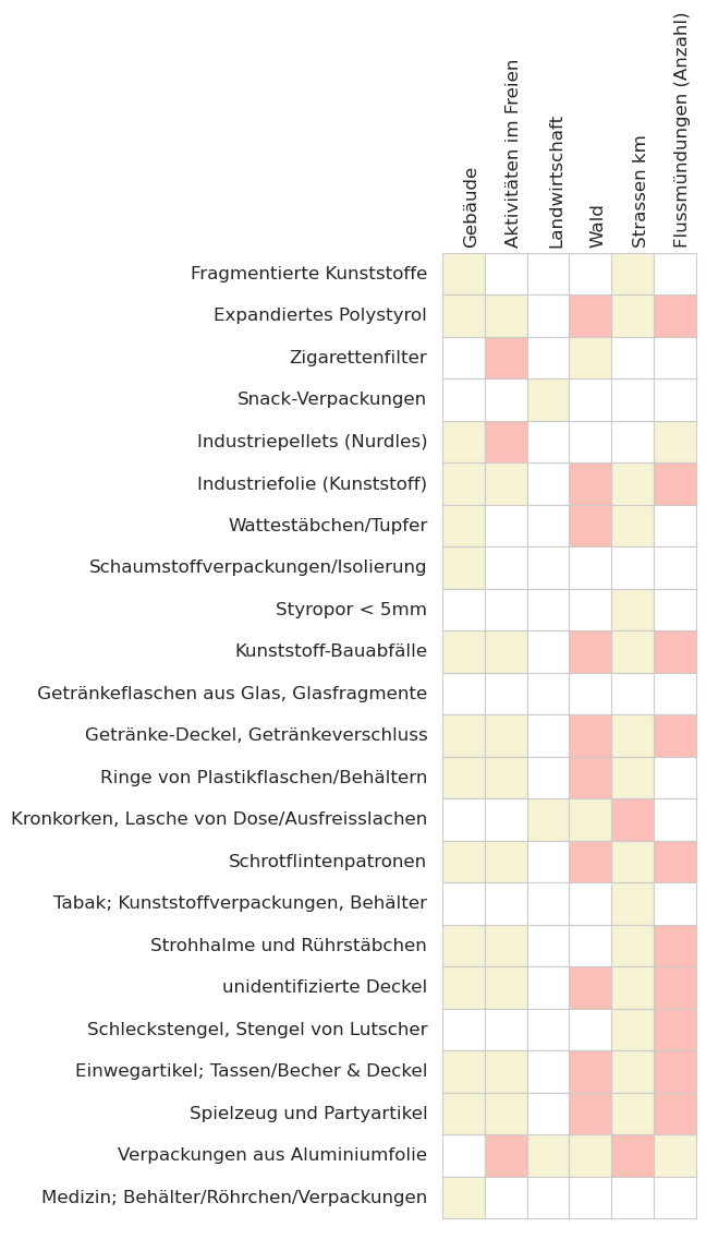
Abb. 5.9

Abbildung 5.9: Ausgewertete Korrelationen der am häufigsten gefundenen Objekte in Bezug auf das Landnutzungsprofil im Erhebungsgebiet Rhône. Für alle gültigen Erhebungen an Seen n=106. Legende: wenn p > 0,05 = weiss, wenn p < 0,05 und Rho > 0 = rot, wenn p < 0,05 und Rho < 0 = gelb.

5.4. Verwendungszweck der gefundenen Objekte

Der Verwendungszweck basiert auf der Verwendung des Objekts, bevor es weggeworfen wurde, oder auf der Artikelbeschreibung, wenn die ursprüngliche Verwendung unbestimmt ist. Identifizierte Objekte werden einer der 260 vordefinierten Kategorien zugeordnet. Die Kategorien werden je nach Verwendung oder Artikelbeschreibung gruppiert.

• Abwasser: Objekte, die aus Kläranlagen freigesetzt werden, sprich Objekte, die wahrscheinlich über die Toilette entsorgt werden

• Mikroplastik (< 5 mm): fragmentierte Kunststoffe und Kunststoffharze aus der Vorproduktion

• Infrastruktur: Artikel im Zusammenhang mit dem Bau und der Instandhaltung von Gebäuden, Strassen und der Wasser-/Stromversorgung

• Essen und Trinken: alle Materialien, die mit dem Konsum von Essen und Trinken in Zusammenhang stehen

• Landwirtschaft: Materialien z. B. für Mulch und Reihenabdeckungen, Gewächshäuser, Bodenbegasung, Ballenverpackungen. Einschliesslich Hartkunststoffe für landwirtschaftliche Zäune, Blumentöpfe usw.

• Tabakwaren: hauptsächlich Zigarettenfilter, einschliesslich aller mit dem Rauchen verbundenen Materialien

• Freizeit und Erholung: Objekte, die mit Sport und Freizeit zu tun haben, z. B. Angeln, Jagen, Wandern usw.

• Verpackungen ausser Lebensmittel und Tabak: Verpackungsmaterial, das nicht lebensmittel- oder tabakbezogen ist

• Plastikfragmente: Plastikteile unbestimmter Herkunft oder Verwendung

• Persönliche Gegenstände: Accessoires, Hygieneartikel und Kleidung

Im Anhang befindet sich die vollständige Liste der identifizierten Objekte, einschliesslich Beschreibungen und Gruppenklassifizierung. Das Kapitel 16 Codegruppen beschreibt jede Codegruppe im Detail und bietet eine umfassende Liste aller Objekte in einer Gruppe.

Show code cell source Hide code cell source

# the results are a callable for the components
components = fdx.componentCodeGroupResults()

# pivot that and reomve any hierarchal column index
pt_comp = components[[this_level, "groupname", '% of total' ]].pivot(columns=this_level, index="groupname")
pt_comp.columns = pt_comp.columns.get_level_values(1)
pt_comp.rename(columns = proper_column_names, inplace=True)

# the aggregated codegroup results from the feature
pt_feature = fdx.codegroup_summary["% of total"]
pt_comp[this_feature["name"]] = pt_feature

# the aggregated totals for the period
pt_period = period_data.parentGroupTotals(parent=False, percent=True)
pt_comp[top] = pt_period

# caption
code_group_percent_caption = [
    'Verwendungszweck oder Beschreibung der identifizierten Objekte in % der ',
    f'Gesamtzahl nach Gemeinden im Erhebungsgebiet {this_feature["name"]}. '
    'Fragmentierte Objekte, die nicht eindeutig identifiziert werden können, ',
    'werden weiterhin nach ihrer Grösse klassifiziert.'
]

code_group_percent_caption = ''.join(code_group_percent_caption)

# format for data frame
pt_comp.index.name = None
pt_comp.columns.name = None
aformatter = {x: '{:.0%}' for x in pt_comp.columns}
ptd = pt_comp.style.format(aformatter).set_table_styles(heat_map_css_styles).background_gradient(axis=None, vmin=pt_comp.min().min(), vmax=pt_comp.max().max(), cmap="YlOrBr")
ptd = ptd.applymap_index(featuredata.rotateText, axis=1)

# the caption prefix is used in the case where the table needs to be split horzontally
caption_prefix =  'Verwendungszweck oder Beschreibung der identifizierten Objekte in % der Gesamtzahl nach Gemeinden: '

col_widths = [4.5*cm, *[1*cm]*(len(pt_comp.columns))]
cgpercent_tables = featuredata.splitTableWidth(pt_comp.mul(100).astype(int), gradient=True, caption_prefix=caption_prefix, caption= code_group_percent_caption,
                    this_feature=this_feature["name"], vertical_header=True, colWidths=col_widths, rowends=-2)

if isinstance(tables, (list, np.ndarray)):
    grouped_pdf_components = [*tables]
else:
    grouped_pdf_components = [tables]


glue("rhone_codegroup_percent_caption", code_group_percent_caption, display=False)
glue("rhone_codegroup_percent", ptd, display=False)

	Lac Léman	Rhône	Erhebungsgebiet Rhône	Alle Erhebungsgebiete
Abwasser	6%	21%	6%	5%
Essen und Trinken	18%	21%	18%	19%
Freizeit und Erholung	4%	2%	4%	4%
Infrastruktur	22%	12%	22%	18%
Landwirtschaft	5%	14%	5%	6%
Mikroplastik (< 5mm)	11%	3%	10%	8%
Persönliche Gegenstände	2%	6%	2%	3%
Plastikfragmente	15%	1%	15%	14%
Tabakwaren	13%	5%	12%	17%
Verpackungen ohne Lebensmittel/Tabak	3%	13%	4%	5%
nicht klassifiziert	1%	2%	1%	1%

Abb. 5.10

Abbildung 5.10: Verwendungszweck oder Beschreibung der identifizierten Objekte in % der Gesamtzahl nach Gemeinden im Erhebungsgebiet Erhebungsgebiet Rhône. Fragmentierte Objekte, die nicht eindeutig identifiziert werden können, werden weiterhin nach ihrer Grösse klassifiziert.

Show code cell source Hide code cell source

# pivot that
grouppcs_comp = components[[this_level, "groupname", unit_label ]].pivot(columns=this_level, index="groupname")

# quash the hierarchal column index
grouppcs_comp.columns = grouppcs_comp.columns.get_level_values(1)
grouppcs_comp.rename(columns = proper_column_names, inplace=True)

# the aggregated codegroup results from the feature
pt_feature = fdx.codegroup_summary[unit_label]
grouppcs_comp[this_feature["name"]] = pt_feature

# the aggregated totals for the period
pt_period = period_data.parentGroupTotals(parent=False, percent=False)
grouppcs_comp[top] = pt_period

# color gradient of restults
code_group_pcsm_gradient = featuredata.colorGradientTable(grouppcs_comp)
grouppcs_comp.index.name = None
grouppcs_comp.columns.name = None

# pdf and display output
code_group_pcsm_caption = [
    f'Verwendungszweck der gefundenen Objekte Median {unit_label} am ',
    f'{this_feature["name"]}. Fragmentierte Objekte, die nicht eindeutig ',
    'identifiziert werden können, werden weiterhin nach ihrer Grösse klassifiziert.'
]
code_group_pcsm_caption = ''.join(code_group_pcsm_caption)

caption_prefix =  f'Verwendungszweck der gefundenen Objekte Median {unit_label} am '
col_widths = [4.5*cm, *[1*cm]*(len(grouppcs_comp.columns))]
cgpcsm_tables = featuredata.splitTableWidth(grouppcs_comp, gradient=True, caption_prefix=caption_prefix, caption=code_group_pcsm_caption,
                    this_feature=this_feature["name"], vertical_header=True, colWidths=col_widths)

if isinstance(cgpcsm_tables, (list, np.ndarray)):
    new_components = [
        featuredata.large_space,
        *cgpercent_tables,    
        featuredata.larger_space,
        *cgpcsm_tables,
        featuredata.larger_space
    ]
else:
    new_components = [
    featuredata.large_space,
    cgpercent_tables,    
    featuredata.larger_space,
    cgpcsm_tables,
    featuredata.larger_space
    ]
    
pdfcomponents = addToDoc(new_components, pdfcomponents)

aformatter = {x: featuredata.replaceDecimal for x in grouppcs_comp.columns}
cgp = grouppcs_comp.style.format(aformatter).set_table_styles(heat_map_css_styles).background_gradient(axis=None, vmin=grouppcs_comp.min().min(), vmax=grouppcs_comp.max().max(), cmap="YlOrBr")
cgp= cgp.applymap_index(featuredata.rotateText, axis=1)


glue("rhone_codegroup_pcsm_caption", code_group_pcsm_caption, display=False)
glue("rhone_codegroup_pcsm", cgp, display=False)

	Lac Léman	Rhône	Erhebungsgebiet Rhône	Alle Erhebungsgebiete
Abwasser	19,5	7,5	19,0	3,0
Essen und Trinken	87,5	12,5	76,0	37,0
Freizeit und Erholung	19,0	4,0	16,5	6,0
Infrastruktur	71,5	12,0	55,5	20,0
Landwirtschaft	14,0	20,5	14,0	7,0
Mikroplastik (< 5mm)	16,0	0,0	11,5	1,0
Persönliche Gegenstände	10,0	11,5	10,0	6,0
Plastikfragmente	61,5	0,5	48,0	18,0
Tabakwaren	52,0	0,0	50,0	25,0
Verpackungen ohne Lebensmittel/Tabak	13,0	14,0	13,0	9,0
nicht klassifiziert	2,0	0,5	2,0	0,0

Abb. 5.11

Abbildung 5.11: Verwendungszweck der gefundenen Objekte Median p/100 m am Erhebungsgebiet Rhône. Fragmentierte Objekte, die nicht eindeutig identifiziert werden können, werden weiterhin nach ihrer Grösse klassifiziert.

5.5. Fliessgewässer

Show code cell source Hide code cell source

# summary of sample totals
csx = fdr.sample_summary.copy()
combined_summary =[(x, featuredata.thousandsSeparator(int(csx[x]), language)) for x in csx.index]

# the lake and river sample totals
rivers = fdr.sample_totals
lakes = fdx.sample_totals

# make the charts
fig = plt.figure(figsize=(11,6))

aspec = fig.add_gridspec(ncols=11, nrows=3)

ax = fig.add_subplot(aspec[:, :6])

line_label = F"{rate} median:{top}"

sns.scatterplot(data=lakes, x="date", y=unit_label, color="black", alpha=0.4, label="Seen", ax=ax)
sns.scatterplot(data=rivers, x="date", y=unit_label, color="red", s=34, ec="white",label="Fliessgewässer", ax=ax)

ax.set_ylabel(unit_label, labelpad=10, fontsize=14)

ax.set_xlabel("")
ax.xaxis.set_minor_locator(days)
ax.xaxis.set_major_formatter(months_fmt)
# ax.margins(x=.05, y=.05)
ax.set_ylim(-50, 2000)

a_col = [this_feature["name"], "Total"]

axone = fig.add_subplot(aspec[:, 6:])
featuredata.hide_spines_ticks_grids(axone)

table_five = sut.make_a_table(axone, combined_summary,  colLabels=a_col, colWidths=[.75,.25],  bbox=[0,0,1,1], **{"loc":"lower center"})
table_five.get_celld()[(0,0)].get_text().set_text(" ")
table_five.set_fontsize(12)

rivers_caption = [
    f'Links: {this_feature["name"]} Fliessgewässer, {featuredata.dateToYearAndMonth(datetime.strptime(start_date, date_format), lang=date_lang)} ',
    f'bis {featuredata.dateToYearAndMonth(datetime.strptime(end_date, date_format), lang=date_lang)}, n = {len(rivers.loc_date.unique())}. ',
    'Rechts: Zusammenfassung der Daten.'
]

rivers_caption = ''.join(rivers_caption)


figure_name = f'{this_feature["slug"]}river_sample_totals'
river_totals_file_name = f'{save_fig_prefix}{figure_name}.jpeg'
save_figure_kwargs.update({"fname":river_totals_file_name})

plt.tight_layout()
plt.savefig(**save_figure_kwargs)

glue('rhone_survey_area_rivers_summary_caption', rivers_caption, display=False)

glue('rhone_survey_area_rivers_summary', fig, display=False)
plt.close()

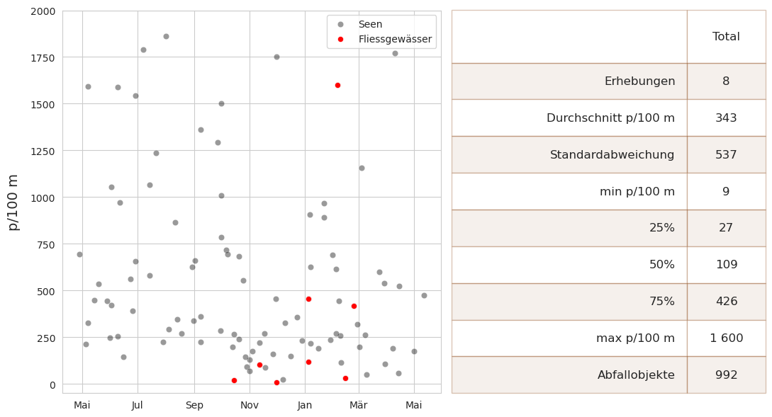
Abb. 5.12

Abbildung 5.12: Links: Erhebungsgebiet Rhône Fliessgewässer, April 2020 bis März 2021, n = 8. Rechts: Zusammenfassung der Daten.

5.5.1. Die an Fliessgewässern am häufigsten gefundenen Objekte

Show code cell source Hide code cell source

# the most common objects results
most_common_display = fdr.most_common.copy()

# language appropriate columns
cols_to_use = featuredata.most_common_objects_table_de
cols_to_use.update({unit_label:unit_label})

# data for display
most_common_display.rename(columns=cols_to_use, inplace=True)
most_common_display = most_common_display[cols_to_use.values()].copy()
most_common_display = most_common_display.set_index("Objekte", drop=True)

# .pdf output
data = most_common_display.copy()
data["Anteil"] = data["Anteil"].map(lambda x: f"{int(x)}%")
data['Objekte (St.)'] = data['Objekte (St.)'].map(lambda x:featuredata.thousandsSeparator(x, language))
data['Häufigkeitsrate'] = data['Häufigkeitsrate'].map(lambda x: f"{x}%")
data[unit_label] = data[unit_label].map(lambda x: featuredata.replaceDecimal(round(x,1)))

# make caption
# get percent of total to make the caption string
m_common_percent_of_total = fdx.most_common['Objekte (St.)'].sum()/fdx.code_summary['quantity'].sum()

mc_caption_string = f'Häufigste Objekte p/100 m an Fliessgewässern im {this_feature["name"]}: Medianwert der Erhebung.'


# pdf_mc_table  = featuredata.aStyledTable(data, caption=mc_caption_string, colWidths=[4.5*cm, 2.2*cm, 2*cm, 2.8*cm, 2*cm])

col_widths = [4.5*cm, 2.2*cm, 2*cm, 2.8*cm, 2*cm]

d_chart = aSingleStyledTable(data, vertical_header=False, gradient=False, colWidths=col_widths)
d_capt = featuredata.makeAParagraph([monthly_data_caption], style=caption_style)
pdf_mc_table = tableAndCaption(d_chart, d_capt, colwidths)

most_common_display.index.name = None
most_common_display.columns.name = None

# set pandas display
aformatter = {
    "Anteil":lambda x: f"{int(x)}%",
    f"{unit_label}": lambda x: featuredata.replaceDecimal(x, language),
    "Häufigkeitsrate": lambda x: f"{int(x)}%",   
    "Objekte (St.)": lambda x: featuredata.thousandsSeparator(int(x), language)
}

mcd = most_common_display.style.format(aformatter).set_table_styles(table_css_styles)
glue('rhone_rivers_most_common_caption', mc_caption_string, display=False)
glue('rhone_rivers_most_common_tables', mcd, display=False)

	Objekte (St.)	Anteil	Häufigkeitsrate	p/100 m
Windeln – Feuchttücher	182	18%	62%	4,0
Industriefolie (Kunststoff)	122	12%	62%	18,0
Snack-Verpackungen	58	5%	50%	1,0
Verpackungsfolien, nicht für Lebensmittel	54	5%	37%	0,0
Zigarettenfilter	53	5%	37%	0,0
Einkaufstaschen, Shoppingtaschen	50	5%	50%	3,5
Getränkeflaschen aus Glas, Glasfragmente	44	4%	12%	0,0
Kronkorken, Lasche von Dose/Ausfreisslachen	42	4%	25%	0,0
Baumaterial; Ziegel, Rohre, Zement	36	3%	12%	0,0
Kunststoff-Bauabfälle	30	3%	50%	3,5
Fragmentierte Kunststoffe	8	0%	50%	0,5

Abb. 5.13

Abbildung 5.13: Häufigste Objekte p/100 m an Fliessgewässern im Erhebungsgebiet Rhône: Medianwert der Erhebung.

5.6. Anhang

5.6.1. Schaumstoffe und Kunststoffe nach Grösse

Die folgende Tabelle enthält die Komponenten «Gfoam» und «Gfrag», die für die Analyse gruppiert wurden. Objekte, die als Schaumstoffe gekennzeichnet sind, werden als Gfoam gruppiert und umfassen alle geschäumten Polystyrol-Kunststoffe > 0,5 cm. Kunststoffteile und Objekte aus kombinierten Kunststoff- und Schaumstoffmaterialien > 0,5 cm werden für die Analyse als Gfrags gruppiert.

Show code cell source Hide code cell source

annex_title = Paragraph("Anhang", section_title)
frag_sub_title = Paragraph("Schaumstoffe und Kunststoffe nach Grösse", subsection_title)

frag_paras = [
    "Die folgende Tabelle enthält die Komponenten «Gfoam» und «Gfrag», die für die Analyse gruppiert wurden. ",
    "Objekte, die als Schaumstoffe gekennzeichnet sind, werden als Gfoam gruppiert und umfassen alle geschäumten ",
    "Polystyrol-Kunststoffe > 0,5 cm. Kunststoffteile und Objekte aus kombinierten Kunststoff - und Schaumstoffmaterialien > 0,5 ",
    "cm werden für die Analyse als Gfrags gruppiert."
]

frag_p = "".join(frag_paras)
frag = Paragraph(frag_p, featuredata.p_style)

frag_caption = [
    f'Fragmentierte und geschäumte Kunststoffe nach Grösse am {this_feature["name"]}',
    f'Median {unit_label}, Anzahl der gefundenen Objekte und Prozent der Gesamtmenge.'
]
frag_captions = ''.join(frag_caption)

# collect the data before aggregating foams for all locations in the survye area
# group by loc_date and code
# Combine the different sizes of fragmented plastics and styrofoam
# the codes for the foams
before_agg = pd.read_csv("resources/checked_before_agg_sdata_eos_2020_21.csv")
some_foams = ["G81", "G82", "G83", "G74"]
before_agg.rename(columns={"p/100m":unit_label}, inplace=True)

# the codes for the fragmented plastics
some_frag_plas = list(before_agg[before_agg.groupname == "plastic pieces"].code.unique())
mask = ((before_agg.code.isin([*some_frag_plas, *some_foams]))&(before_agg.location.isin(admin_summary["locations_of_interest"])))
agg_pcs_median = {unit_label:"median", "quantity":"sum"}

fd_frags_foams = before_agg[mask].groupby(["loc_date","code"], as_index=False).agg(agg_pcs_quantity)
fd_frags_foams = fd_frags_foams.groupby("code").agg(agg_pcs_median)
fd_frags_foams["item"] = fd_frags_foams.index.map(lambda x: fdx.dMap.loc[x])
fd_frags_foams["% of total"] = (fd_frags_foams.quantity/fd.quantity.sum()).round(2)

# table data
data = fd_frags_foams[["item",unit_label, "quantity", "% of total"]]
data.rename(columns={"item":"Objekt", "quantity":"Objekte (St.)", "% of total":"Anteil"}, inplace=True)
data.set_index("Objekt", inplace=True, drop=True)
data.index.name = None

aformatter = {
    f"{unit_label}": lambda x: featuredata.replaceDecimal(x, language),
    "Objekte (St.)": lambda x: featuredata.thousandsSeparator(int(x), language),
    "Anteil":'{:.0%}'   
}

frags_table = data.style.format(aformatter).set_table_styles(table_css_styles)

glue("rhone_frag_table_caption", frag_captions, display=False)
glue("rhone_frags_table", frags_table, display=False)

# frag_table = featuredata.aStyledTable(data, caption=frag_captions, colWidths=[7*cm, *[2*cm]*(len(dims_table.columns)-1)])
col_widths = [7*cm, *[2*cm]*(len(data.columns)-1)]

d_chart = aSingleStyledTable(data, vertical_header=False, gradient=False, colWidths=col_widths)
d_capt = featuredata.makeAParagraph(frag_caption, style=caption_style)
pdf_mc_table = tableAndCaption(d_chart, d_capt, colwidths)

new_components = [
    KeepTogether([
        annex_title,
        small_space,
        frag_sub_title,
        featuredata.smaller_space,
        frag,
        small_space
    ]),
    pdf_mc_table
]

pdfcomponents = addToDoc(new_components, pdfcomponents)

	p/100 m	Objekte (St.)	Anteil
Schaumstoffverpackungen/Isolierung	0,0	121	0%
Objekte aus Kunststoff/Polystyrol 0,5 - 2,5 cm	0,0	443	2%
Objekte aus Kunststoff/Polystyrol 2,5 - 50 cm	0,0	83	0%
Objekte aus Kunststoff 0,5 - 2,5 cm	18,0	2 035	7%
Objekte aus Kunststoff 2,5 - 50 cm	12,5	1 659	6%
Objekte aus Kunststoff > 50 cm	0,0	0	0%
Objekte aus expandiertem Polystyrol 0,5 - 2,5 cm	6,0	2 476	9%
Objekte aus expandiertem Polystyrol 2,5 - 50 cm	4,0	1 108	4%
Objekte aus expandiertem Polystyrol > 50 cm	0,0	5	0%

Abb. 5.14

Abbildung 5.14: Fragmentierte und geschäumte Kunststoffe nach Grösse am Erhebungsgebiet RhôneMedian p/100 m, Anzahl der gefundenen Objekte und Prozent der Gesamtmenge.

5.6.2. Die Erhebungsorte

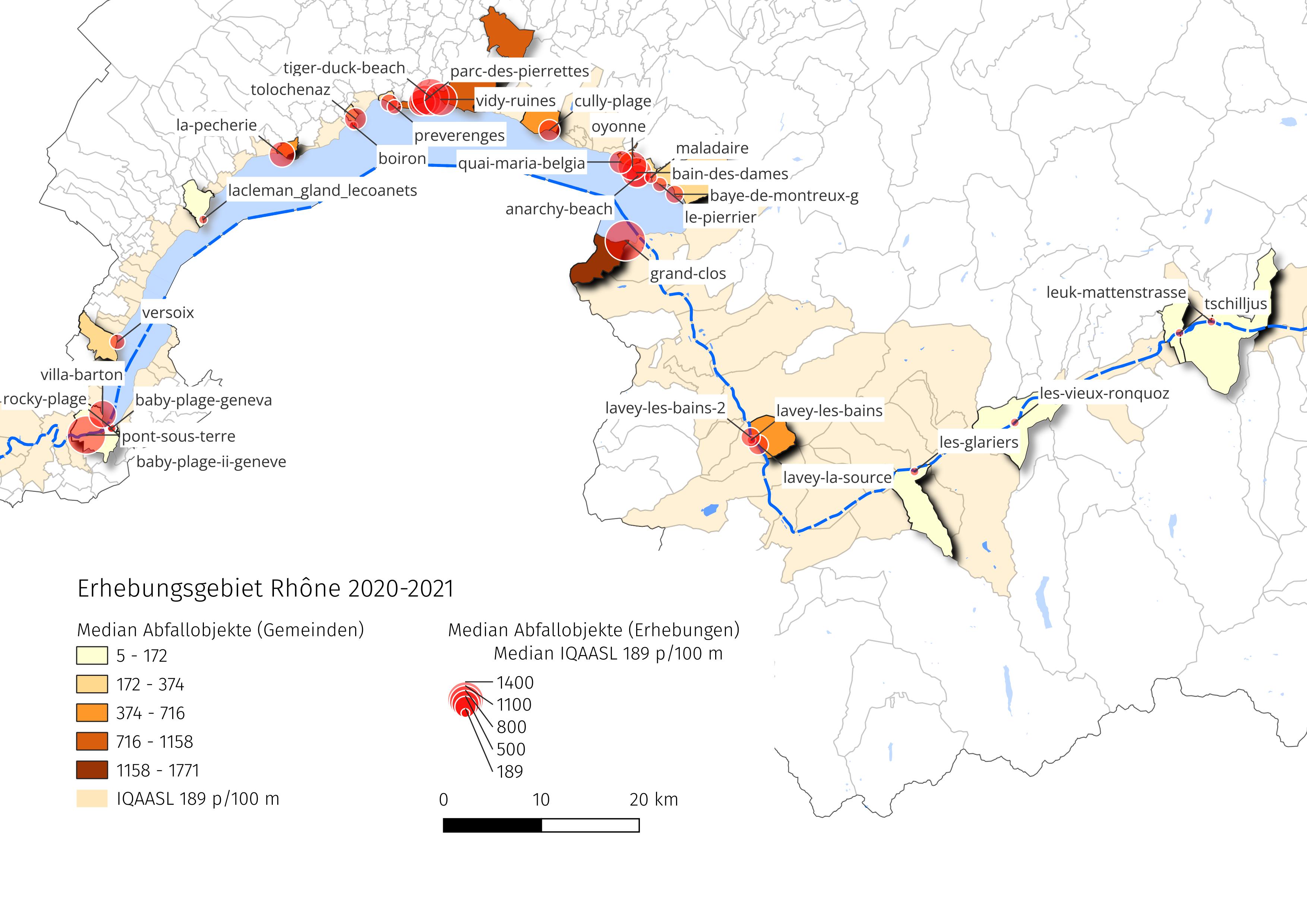
Abb. 5.15

Show code cell source Hide code cell source

# display the survey locations
disp_columns = ["latitude", "longitude", "city"]
disp_beaches = admin_details.df_beaches.loc[admin_summary["locations_of_interest"]][disp_columns]
disp_beaches.reset_index(inplace=True)
disp_beaches.rename(columns={"city":"stat", "slug":"standort"}, inplace=True)
disp_beaches.set_index("standort", inplace=True, drop=True)

# make this into a pdf table
location_subsection = Paragraph("Die Erhebungsorte und Inventar der Objekte", subsection_title)
col_widths = [6*cm, 2.2*cm, 2.2*cm, 3*cm]
pdf_table = aStyledTableWithTitleRow(disp_beaches, title="Die Erhebungsorte", colWidths=col_widths)

disp_beaches

	latitude	longitude	stat
standort
maladaire	46.446296	6.876960	La Tour-de-Peilz
preverenges	46.512690	6.527657	Préverenges
vidy-ruines	46.516221	6.596279	Lausanne
baby-plage-geneva	46.208558	6.162923	Genève
grand-clos	46.387746	6.843686	Saint-Gingolph
quai-maria-belgia	46.460156	6.836718	Vevey
anarchy-beach	46.447216	6.859612	La Tour-de-Peilz
lavey-les-bains-2	46.207726	7.011685	Lavey-Morcles
leuk-mattenstrasse	46.314754	7.622521	Leuk
pont-sous-terre	46.202960	6.131577	Genève
cully-plage	46.488887	6.741396	Bourg-en-Lavaux
preverenges-le-sout	46.508905	6.534526	Préverenges
la-pecherie	46.463919	6.385732	Allaman
villa-barton	46.222350	6.152500	Genève
oyonne	46.456682	6.852262	La Tour-de-Peilz
lavey-la-source	46.200804	7.021866	Lavey-Morcles
lavey-les-bains	46.205159	7.012722	Lavey-Morcles
baby-plage-ii-geneve	46.208940	6.164330	Genève
les-glariers	46.176736	7.228925	Riddes
tiger-duck-beach	46.518256	6.582546	Saint-Sulpice (VD)
le-pierrier	46.439727	6.888968	Montreux
tschilljus	46.304399	7.580262	Salgesch
boiron	46.491030	6.480162	Tolochenaz
rocky-plage	46.209737	6.164952	Genève
lacleman_gland_lecoanets	46.402811	6.281959	Gland
baye-de-montreux-g	46.430834	6.908778	Montreux
les-vieux-ronquoz	46.222049	7.361664	Sion
versoix	46.289194	6.170569	Versoix
parc-des-pierrettes	46.515215	6.575531	Saint-Sulpice (VD)
plage-de-st-sulpice	46.513265	6.570977	Saint-Sulpice (VD)
bain-des-dames	46.450507	6.858092	La Tour-de-Peilz
tolochenaz	46.497509	6.482875	Tolochenaz

5.6.3. Inventar der Objekte

Show code cell source Hide code cell source

pd.set_option("display.max_rows", None)
complete_inventory = fdx.code_summary.copy()
complete_inventory.sort_values(by="quantity", ascending=False, inplace=True)
complete_inventory["quantity"] = complete_inventory["quantity"].map(lambda x: featuredata.thousandsSeparator(x, language))
complete_inventory["% of total"] = complete_inventory["% of total"].astype(int)
complete_inventory[unit_label] = complete_inventory[unit_label].astype(int)
complete_inventory.rename(columns=featuredata.inventory_table_de, inplace=True)
    
inventory_subsection = Paragraph("Inventar der Objekte", subsection_title)
col_widths=[1.2*cm, 4.5*cm, 2.2*cm, 1.5*cm, 1.5*cm, 2.4*cm, 1.5*cm]
inventory_table = aStyledTableWithTitleRow(complete_inventory, title="Inventar der Objekte", colWidths=col_widths)

new_map_image =  Image('resources/maps/rhone_location_labels.jpeg', width=cm*16, height=12*cm, kind="proportional", hAlign= "CENTER")
new_components = [
    KeepTogether([
        featuredata.large_space,
        location_subsection,
        small_space,
        new_map_image,
        Paragraph(map_caption, caption_style),
        featuredata.smaller_space,
        pdf_table,
        
    ]),
    featuredata.large_space,
    inventory_table
]    

pdfcomponents = addToDoc(new_components, pdfcomponents)

complete_inventory

	Objekte	Objekte (St.)	Anteil	p/100 m	Häufigkeitsrate	Material
code
Gfrags	Fragmentierte Kunststoffe	4 220	14	48	93	Plastik
Gfoam	Expandiertes Polystyrol	3 589	12	17	80	Plastik
G27	Zigarettenfilter	3 169	11	41	90	Plastik
G30	Snack-Verpackungen	1 737	6	19	92	Plastik
G112	Industriepellets (Nurdles)	1 387	4	0	43	Plastik
G67	Industriefolie (Kunststoff)	1 180	4	9	76	Plastik
G95	Wattestäbchen/Tupfer	1 112	3	10	75	Plastik
G74	Schaumstoffverpackungen/Isolierung	1 112	3	7	71	Plastik
G117	Styropor < 5mm	718	2	0	28	Plastik
G89	Kunststoff-Bauabfälle	614	2	5	65	Plastik
G200	Getränkeflaschen aus Glas, Glasfragmente	554	1	2	54	Glas
G106	Kunststofffragmente eckig <5mm	427	1	0	22	Plastik
G21	Getränke-Deckel, Getränkeverschluss	425	1	1	51	Plastik
G24	Ringe von Plastikflaschen/Behältern	362	1	4	68	Plastik
G178	Kronkorken, Lasche von Dose/Ausfreisslachen	350	1	3	67	Metall
G70	Schrotflintenpatronen	347	1	0	50	Plastik
G25	Tabak; Kunststoffverpackungen, Behälter	296	1	1	51	Plastik
G98	Windeln – Feuchttücher	295	1	0	35	Plastik
G10	Lebensmittelbehälter zum einmaligen Gebrauch a...	288	1	0	47	Plastik
G35	Strohhalme und Rührstäbchen	278	0	3	67	Plastik
G23	unidentifizierte Deckel	263	0	2	54	Plastik
G31	Schleckstengel, Stengel von Lutscher	238	0	2	62	Plastik
G103	Kunststofffragmente rund <5mm	229	0	0	5	Plastik
G3	Einkaufstaschen, Shoppingtaschen	206	0	0	24	Plastik
G33	Einwegartikel; Tassen/Becher & Deckel	201	0	2	55	Plastik
G32	Spielzeug und Partyartikel	194	0	2	60	Plastik
G177	Verpackungen aus Aluminiumfolie	178	0	1	52	Metall
G100	Medizin; Behälter/Röhrchen/Verpackungen	177	0	2	57	Plastik
G921	Keramikfliesen und Bruchstücke	176	0	0	23	Glas
G22	Deckel für Chemikalien, Reinigungsmittel (Ohne...	176	0	0	31	Plastik
G73	Gegenstände aus Schaumstoff & Teilstücke (nich...	166	0	0	38	Plastik
G38	Abdeckungen; Kunststoffverpackungen, Folien zu...	152	0	0	11	Plastik
G941	Verpackungsfolien, nicht für Lebensmittel	139	0	0	17	Plastik
G66	Umreifungsbänder; Hartplastik für Verpackung f...	135	0	0	41	Plastik
G211	Sonstiges medizinisches Material	103	0	0	41	Plastik
G156	Papierfragmente	101	0	0	25	Papier
G922	Etiketten, Strichcodes	99	0	0	31	Plastik
G91	Bio-Filtermaterial / Trägermaterial aus Kunst...	96	0	0	34	Plastik
G159	Kork	90	0	0	38	Holz
G208	Glas oder Keramikfragmente >2.5 cm	87	0	0	14	Glas
G904	Feuerwerkskörper; Raketenkappen	85	0	0	23	Plastik
G90	Blumentöpfe aus Plastik	80	0	0	25	Plastik
G125	Luftballons und Luftballonstäbchen	79	0	0	26	Gummi
G96	Hygienebinden/Höscheneinlagen/Tampons und Appl...	77	0	0	30	Plastik
G204	Baumaterial; Ziegel, Rohre, Zement	68	0	0	15	Glas
G165	Glacestengel (Eisstiele), Zahnstocher, Essstäb...	68	0	0	22	Holz
G124	Andere Kunststoff	68	0	0	16	Plastik
G914	Büroklammern, Wäscheklammern, Gebrauchsgegenst...	65	0	0	24	Plastik
G34	Besteck, Teller und Tabletts	65	0	0	25	Plastik
G50	Schnur < 1cm	62	0	0	29	Plastik
G153	Papierbecher, Lebensmittelverpackungen aus Pap...	62	0	0	17	Papier
G105	Kunststofffragmente subangulär <5mm	59	0	0	7	Plastik
G908	Klebeband; elektrisch, isolierend	58	0	0	19	Plastik
G198	Andere Metallteile < 50 cm	58	0	0	25	Metall
G28	Stifte, Deckel, Druckbleistifte usw.	57	0	0	28	Plastik
G137	Kleidung, Handtücher und Lappen	54	0	0	17	Stoff
G923	Taschentücher, Toilettenpapier, Servietten, Pa...	51	0	0	18	Papier
G93	Kabelbinder	51	0	0	24	Plastik
G149	Papierverpackungen	50	0	0	13	Papier
G905	Haarspangen, Haargummis, persönliche Accessoir...	48	0	0	29	Plastik
G26	Feuerzeug	45	0	0	22	Plastik
G155	Feuerwerkspapierhülsen und -fragmente	44	0	0	2	Papier
G131	Gummibänder	43	0	0	26	Gummi
G115	Schaumstoff <5mm	43	0	0	3	Plastik
G146	Papier, Karton	40	0	0	9	Papier
G152	Papier &Karton;Zigarettenschachteln, Papier/Ka...	39	0	0	13	Papier
G937	Pheromonköder für Weinberge	38	0	0	16	Plastik
G7	Getränkeflaschen < = 0,5 l	35	0	0	14	Plastik
G157	Papier	35	0	0	10	Papier
G939	Kunststoffblumen, Kunststoffpflanzen	33	0	0	13	Plastik
G4	Kleine Plastikbeutel; Gefrierbeutel, Zippsäckc...	33	0	0	13	Plastik
G20	Laschen und Deckel	31	0	0	12	Plastik
G135	Kleidung, Fussbekleidung, Kopfbedeckung, Hands...	31	0	0	15	Stoff
G142	Seil, Schnur oder Netze	30	0	0	15	Stoff
G207	Tonkrüge zum Fangen von Kraken	30	0	0	0	Glas
G191	Draht und Gitter	29	0	0	13	Metall
G65	Eimer	28	0	0	13	Plastik
G175	Getränkedosen (Dosen, Getränke)	28	0	0	12	Metall
G213	Paraffinwachs	28	0	0	17	Chemikalien
G144	Tampons	27	0	0	10	Stoff
G12	Kosmetika, Behälter für Körperpflegeprodukte, ...	25	0	0	13	Plastik
G148	Kartonkisten und Stücke	23	0	0	6	Papier
G48	Seile, synthetische	23	0	0	14	Plastik
G99	Spritzen - Nadeln	21	0	0	16	Plastik
G2	Säcke, Taschen	20	0	0	10	Plastik
G134	Sonstiges Gummi	20	0	0	13	Gummi
G936	Folien für Gewächshäuser	20	0	0	10	Plastik
G943	Zäune Landwirtschaft, Kunststoff	19	0	0	8	Plastik
G114	Folien <5mm	18	0	0	1	Plastik
G6	Flaschen und Behälter aus Kunststoff, nicht fü...	18	0	0	5	Plastik
G8	Getränkeflaschen > 0,5L	17	0	0	8	Plastik
G194	Kabel, Metalldraht oft in Gummi- oder Kunststo...	17	0	0	15	Metall
G126	Bälle	17	0	0	10	Gummi
G123	Polyurethan-Granulat < 5mm	17	0	0	0	Plastik
G927	Plastikschnur von Rasentrimmern, die zum Schne...	16	0	0	8	Plastik
G87	Abdeckklebeband/Verpackungsklebeband	16	0	0	7	Plastik
G918	Sicherheitsnadeln, Büroklammern, kleine Gebrau...	16	0	0	8	Metall
G43	Sicherheitsetiketten, Siegel für Fischerei ode...	15	0	0	5	Plastik
G182	Angeln; Haken, Gewichte, Köder, Senkblei, usw.	15	0	0	7	Metall
G186	Industrieschrott	14	0	0	5	Metall
G203	Geschirr aus Keramik oder Glas, Tassen, Teller...	14	0	0	5	Glas
G113	Fäden <5mm	14	0	0	3	Plastik
G145	Andere Textilien	14	0	0	9	Stoff
G199	Andere Metallteile > 50 cm	13	0	0	3	Metall
G201	Gläser, einschliesslich Stücke	13	0	0	5	Glas
G930	Schaumstoff-Ohrstöpsel	12	0	0	9	Plastik
G59	Monofile Angelschnur (Angeln)	11	0	0	6	Plastik
G170	Holz (verarbeitet)	11	0	0	6	Holz
G901	Medizinische Masken, synthetische	11	0	0	8	Plastik
G928	Bänder und Schleifen	11	0	0	4	Plastik
G64	Kotflügel	11	0	0	1	Plastik
G942	Kunststoffspäne von Drehbänken, CNC-Bearbeitung	10	0	0	7	Plastik
G11	Kosmetika für den Strand, z.B. Sonnencreme	10	0	0	7	Plastik
G158	Sonstige Gegenstände aus Papier	10	0	0	2	Papier
G210	Sonstiges Glas/Keramik Materialien	10	0	0	3	Glas
G940	Schaumstoff EVA (flexibler Kunststoff)	10	0	0	3	Plastik
G931	(Absperr)band für Absperrungen, Polizei, Baust...	10	0	0	4	Plastik
G938	Zahnstocher, Zahnseide Kunststoff	9	0	0	7	Plastik
G176	Konservendosen (Lebensmitteldosen)	9	0	0	4	Metall
G906	Kaffeekapseln Aluminium	8	0	0	3	Metall
G119	Folienartiger Kunststoff (>1mm)	8	0	0	0	Plastik
G926	Kaugummi, enthält oft Kunststoffe	8	0	0	5	Plastik
G133	Kondome einschließlich Verpackungen	8	0	0	6	Gummi
G900	Handschuhe Latex, persönliche Schutzausrüstung	8	0	0	6	Gummi
G118	Kleine Industrielle Kügelchen <5mm	8	0	0	3	Plastik
G128	Reifen und Antriebsriemen	8	0	0	5	Gummi
G101	Robidog Hundekot-Säcklein, andere Hundekotsäck...	8	0	0	7	Plastik
G136	Schuhe	7	0	0	3	Stoff
G36	Säcke aus strapazierfähigem Kunststoff für 25 ...	7	0	0	1	Plastik
G195	Batterien (Haushalt)	7	0	0	6	Metall
G929	Elektronik und Teile; Sensoren, Headsets usw.	7	0	0	5	Metall
G933	Taschen, Etuis für Zubehör, Brillen, Elektroni...	7	0	0	2	Plastik
G68	Fiberglas-Fragmente	7	0	0	5	Plastik
G61	Sonstiges Angelzubehör	7	0	0	5	Plastik
G916	Bleistifte und Bruchstücke	7	0	0	5	Holz
G37	Netzbeutel, Netztasche, Netzsäcke	6	0	0	2	Plastik
G919	Nägel, Schrauben, Bolzen usw.	5	0	0	3	Metall
G917	Blähton	5	0	0	2	Glas
G167	Streichhölzer oder Feuerwerke	5	0	0	2	Holz
G17	Kartuschen von Kartuschen-spritzpistolen	5	0	0	1	Plastik
G19	Autoteile	5	0	0	2	Plastik
G97	Behälter von Toilettenerfrischer	5	0	0	4	Plastik
G147	Papiertragetaschen, (Papiertüten)	5	0	0	4	Papier
G29	Kämme, Bürsten und Sonnenbrillen	4	0	0	3	Plastik
G181	Geschirr aus Metall, Tassen, Besteck usw.	4	0	0	3	Metall
G915	Reflektoren, Mobilitätsartikel aus Kunststoff	4	0	0	3	Plastik
G913	Schnuller	3	0	0	2	Plastik
G116	Granulat <5mm	3	0	0	0	Plastik
G129	Schläuche und Gummiplatten	3	0	0	1	Gummi
G13	Flaschen, Behälter, Fässer zum Transportieren ...	3	0	0	1	Plastik
G92	Köderbehälter	3	0	0	2	Plastik
G63	Bojen	3	0	0	1	Plastik
G161	Verarbeitetes Holz	3	0	0	1	Holz
G197	sonstiges Metall	3	0	0	2	Metall
G108	Scheibenförmige Pellets <5mm	3	0	0	1	Plastik
G104	Kunststofffragmente abgerundet / rundlich <5m...	3	0	0	1	Plastik
G62	Schwimmer für Netze	3	0	0	1	Plastik
G40	Handschuhe Haushalt/Garten	3	0	0	1	Plastik
G109	Flache Pellets <5mm	2	0	0	0	Plastik
G907	Kaffeekapseln aus Kunststoff	2	0	0	1	Plastik
G151	Tetrapack, Kartons	2	0	0	1	Papier
G925	Pakete: Trockenmittel/Feuchtigkeitsabsorber, m...	2	0	0	1	Plastik
G107	Zylindrische Pellets <5mm	2	0	0	0	Plastik
G140	Sack oder Beutel (Tragetasche), Jute oder Hanf	2	0	0	0	Stoff
G139	Rucksäcke	2	0	0	0	Stoff
G150	Milchkartons, Tetrapack	2	0	0	1	Papier
G55	Angelschnur (verwickelt)	2	0	0	1	Plastik
G932	Bio-Beads, Mikroplastik für die Abwasserbehand...	2	0	0	0	Plastik
G49	Seile > 1cm	2	0	0	1	Plastik
G5	Plastiksäcke/ Plastiktüten	2	0	0	1	Plastik
G138	Schuhe und Sandalen	1	0	0	0	Stoff
G174	Aerosolspraydosen	1	0	0	0	Metall
G179	Einweg Grill	1	0	0	0	Metall
G183	Teile von Angelhaken	1	0	0	0	Metall
G185	Behälter mittlerer Grösse	1	0	0	0	Metall
G171	Sonstiges Holz < 50cm	1	0	0	0	Holz
G102	Flip-Flops	1	0	0	0	Plastik
G193	Teile von Autos und Autobatterien	1	0	0	0	Metall
G196	Grosse metallische Gegenstände	1	0	0	0	Metall
G39	Handschuhe	1	0	0	0	Plastik
G202	Glühbirnen	1	0	0	0	Glas
G154	Zeitungen oder Zeitschriften	1	0	0	0	Papier
G172	Sonstiges Holz > 50 cm	1	0	0	0	Holz
G51	Fischernetz	1	0	0	0	Plastik
G9	Flaschen und Behälter für Reinigungsmittel und...	1	0	0	0	Plastik
G935	Gummi-Puffer für Geh- und Wanderstöcke und Tei...	1	0	0	0	Plastik
G945	Rasierklingen	1	0	0	0	Metall
G166	Farbpinsel	1	0	0	0	Holz
G14	Flaschen für Motoröl (Motorölflaschen)	1	0	0	0	Plastik
G173	Sonstiges	1	0	0	0	Holz
G999	Keine Gegenstände bei dieser Erhebung/Studie g...	0	0	0	0	Unbekannt
G111	Kugelförmige Pellets < 5mm	0	0	0	0	Plastik
G94	Tischtuch	0	0	0	0	Plastik
G934	Sandsäcke, Kunststoff für Hochwasser- und Eros...	0	0	0	0	Plastik
G944	Pelletmasse aus dem Spritzgussverfahren	0	0	0	0	Plastik
G160	Paletten	0	0	0	0	Holz
G60	Lichtstab, Knicklicht, Glow-sticks	0	0	0	0	Plastik
G903	Behälter und Packungen für Handdesinfektionsmi...	0	0	0	0	Plastik
G702	Pistenmarkierungspfosten (Holz)	0	0	0	0	Holz
G162	Kisten	0	0	0	0	Holz
G168	Holzbretter	0	0	0	0	Holz
G180	Haushaltsgeräte	0	0	0	0	Metall
G188	Andere Kanister/Behälter < 4 L	0	0	0	0	Metall
G190	Farbtöpfe, Farbbüchsen, ( Farbeimer)	0	0	0	0	Metall
G205	Leuchtstoffröhren	0	0	0	0	Glas
G214	Öl/Teer	0	0	0	0	Chemikalien
G143	Segel und Segeltuch	0	0	0	0	Stoff
G141	Teppiche	0	0	0	0	Stoff
G132	Schwimmer (Angeln)	0	0	0	0	Gummi
G41	Handschuhe Industriell/Professionell	0	0	0	0	Plastik
G52	Netze und Teilstücke	0	0	0	0	Plastik
G53	Netze und Teilstücke < 50cm	0	0	0	0	Plastik
G56	Verhedderte Netze	0	0	0	0	Plastik
G703	Pistenmarkierungspfosten (Plastik)	0	0	0	0	Plastik
G902	Medizinische Masken, Stoff	0	0	0	0	Stoff
G704	Seilbahnbürsten	0	0	0	0	Plastik
G705	Schrauben und Bolzen	0	0	0	0	Metall
G706	Skiabonnement	0	0	0	0	Plastik
G707	Skiausrüstungsetikett	0	0	0	0	Plastik
G708	Skistöcke	0	0	0	0	Metall
G709	Teller von Skistock (runder Teil aus Plastik u...	0	0	0	0	Plastik
G71	Schuhe Sandalen	0	0	0	0	Plastik
G710	Ski / Snowboards (Ski, Befestigungen und ander...	0	0	0	0	Plastik
G711	Handwärmer	0	0	0	0	Plastik
G712	Skihandschuhe	0	0	0	0	Stoff
G713	Skiförderband	0	0	0	0	Plastik
G84	CD oder CD-Hülle	0	0	0	0	Plastik
G88	Telefon inkl. Teile	0	0	0	0	Plastik
G122	Kunststofffragmente (>1mm)	0	0	0	0	Plastik
G1	Sixpack-Ringe	0	0	0	0	Plastik