Alpen und der Jura

Inhalt

Show code cell source Hide code cell source

# -*- coding: utf-8 -*-
# This is a report using the data from IQAASL.
# IQAASL was a project funded by the Swiss Confederation
# It produces a summary of litter survey results for a defined region.
# These charts serve as the models for the development of plagespropres.ch
# The data is gathered by volunteers.
# Please remember all copyrights apply, please give credit when applicable
# The repo is maintained by the community effective January 01, 2022
# There is ample opportunity to contribute, learn and teach
# contact dev@hammerdirt.ch

# Dies ist ein Bericht, der die Daten von IQAASL verwendet.
# IQAASL war ein von der Schweizerischen Eidgenossenschaft finanziertes Projekt.
# Es erstellt eine Zusammenfassung der Ergebnisse der Littering-Umfrage für eine bestimmte Region.
# Diese Grafiken dienten als Vorlage für die Entwicklung von plagespropres.ch.
# Die Daten werden von Freiwilligen gesammelt.
# Bitte denken Sie daran, dass alle Copyrights gelten, bitte geben Sie den Namen an, wenn zutreffend.
# Das Repo wird ab dem 01. Januar 2022 von der Community gepflegt.
# Es gibt reichlich Gelegenheit, etwas beizutragen, zu lernen und zu lehren.
# Kontakt dev@hammerdirt.ch

# Il s'agit d'un rapport utilisant les données de IQAASL.
# IQAASL était un projet financé par la Confédération suisse.
# Il produit un résumé des résultats de l'enquête sur les déchets sauvages pour une région définie.
# Ces tableaux ont servi de modèles pour le développement de plagespropres.ch
# Les données sont recueillies par des bénévoles.
# N'oubliez pas que tous les droits d'auteur s'appliquent, veuillez indiquer le crédit lorsque cela est possible.
# Le dépôt est maintenu par la communauté à partir du 1er janvier 2022.
# Il y a de nombreuses possibilités de contribuer, d'apprendre et d'enseigner.
# contact dev@hammerdirt.ch

# sys, file and nav packages:
import datetime as dt
from datetime import date, datetime, time
from babel.dates import format_date, format_datetime, format_time, get_month_names
import locale

# math packages:
import pandas as pd
import numpy as np
from scipy import stats
from math import pi

# charting:
import matplotlib.pyplot as plt
import matplotlib.dates as mdates
from matplotlib import ticker
from matplotlib.ticker import MultipleLocator
import seaborn as sns

# build report
from reportlab.platypus import SimpleDocTemplate, Paragraph, Image, PageBreak, KeepTogether
from reportlab.lib.pagesizes import A4
from reportlab.lib.units import cm
from reportlab.platypus import Table, TableStyle

# the module that has all the methods for handling the data
import resources.featuredata as featuredata
from resources.featuredata import makeAParagraph, sectionParagraphs, makeAList, block_quote_style

# home brew utitilties
import resources.chart_kwargs as ck
import resources.sr_ut as sut

# images and display
from IPython.display import Markdown as md
from myst_nb import glue

# chart style
sns.set_style("whitegrid")

# colors for gradients
# colors_palette = ck.colors_palette
bassin_pallette = featuredata.bassin_pallette

# border and row shading for tables
# table_row = "saddlebrown"

# a place to save figures and a 
# method to choose formats
save_fig_prefix = "resources/output/"

# the arguments for formatting the image
save_figure_kwargs = {
    "fname": None,
    "dpi": 300.0,
    "format": "jpeg",
    "bbox_inches": None,
    "pad_inches": 0,
    "bbox_inches": 'tight',
    "facecolor": 'auto',
    "edgecolor": 'auto',
    "backend": None,
}


## !! Begin Note book variables !!
# There are two language variants: german and english
# change both: date_lang and language
date_lang =  'de_DE.utf8'
locale.setlocale(locale.LC_ALL, date_lang)

# the date format of the survey data is defined in the module
date_format = featuredata.date_format

# the language setting use lower case: en or de
# changing the language may require changing the unit label
language = "de"
unit_label = "p/100 m"

# the standard date format is "%Y-%m-%d" if your date column is
# not in this format it will not work.
# these dates cover the duration of the IQAASL project
start_date = "2020-03-01"
end_date ="2021-10-31"
start_end = [start_date, end_date]

# the fail rate used to calculate the most common codes is
# 50% it can be changed:
fail_rate = 50

# common aggregations
agg_pcs_quantity = {unit_label:"sum", "quantity":"sum"}
agg_pcs_median = {unit_label:"median", "quantity":"sum"}

bassin_map = "resources/maps/alpesvalaisannes.jpeg"

# the label for the aggregation of all data in the region
# this is the chart label
top = "Alle Erhebungsgebiete"

# define the feature level and components
# the label for charting is called 'name'
this_feature = {'slug':'les-alpes', 'name':"Alpen und Jura", 'level':'river_bassin'}

# these are the smallest aggregated components
# choices are water_name_slug=lake or river, city or location at the scale of a river bassin 
# water body or lake maybe the most appropriate
this_level = 'location'

# location and object data
dfBeaches = pd.read_csv("resources/beaches_with_land_use_rates.csv")
dfCodes = pd.read_csv("resources/codes_with_group_names_2015.csv")

# the dimensional data from each survey
dfDims = pd.read_csv("resources/alpes_dims.csv")

# beach data
dfBeaches.set_index("slug", inplace=True)

# index the code data
dfCodes.set_index("code", inplace=True)

columns={"% to agg":"% agg", "% to recreation": "% recreation", "% to woods":"% woods", "% to buildings":"% buildings", "p/100m":"p/100 m"}

# key word arguments to construct feature data
# !Note the water type allows the selection of river or lakes
# if None then the data is aggregated together. This selection
# is only valid for survey-area reports or other aggregated data
# that may have survey results from both lakes and rivers.
fd_kwargs ={
    "filename": "resources/combined_alps_iqaasl.csv",
    "feature_name": this_feature['slug'], 
    "feature_level": this_feature['level'], 
    "these_features": this_feature['slug'], 
    "component": this_level, 
    "columns": columns, 
    "language": language, 
    "unit_label": unit_label, 
    "fail_rate": fail_rate,
    "code_data":dfCodes,
    "date_range": start_end,
    "water_type": None,    
}

fdx = featuredata.Components(**fd_kwargs)

# call the reports and languages
fdx.adjustForLanguage()
fdx.makeFeatureData()
fdx.locationSampleTotals(columns=["loc_date", "location", "date"])
fdx.makeDailyTotalSummary()
fdx.materialSummary()
fdx.mostCommon()
# !this is the feature data!
fd = fdx.feature_data

# this maps the slug-value to the proper name
proper_names = dfBeaches[dfBeaches.river_bassin == 'les-alpes']["location"]

# a method to map proper name to slug when the proper name is the index
# value of a dataframe.
reverse_name_look_up = dfBeaches[dfBeaches.river_bassin == 'les-alpes']["location"].reset_index()
reverse_name_look_up = reverse_name_look_up.set_index("location")

# the sample totals are calculated by calling locationSampleTotals
# this sets the index to location and allows acces to the sample totals by
# location name instead of date. This is only valid because there is one 
# sample per location.
unit_label_map = fdx.sample_totals[["location", unit_label]].set_index("location")


# the period data is the data from the Iqaasl project
# not collected in the alpes.
mask = fdx.period_data.river_bassin != this_feature["slug"]

period_kwargs = {
    "period_data": fdx.period_data[mask].copy(),
    "these_features": this_feature['slug'],
    "feature_level":this_feature['level'],
    "feature_parent":this_feature['slug'],
    "parent_level": this_feature['level'],
    "period_name": top,
    "unit_label": unit_label,
    "most_common": fdx.most_common.index
}
period_data = featuredata.PeriodResults(**period_kwargs)

# collects the summarized values for the feature data
# use this to generate the summary data for the survey area
# and the section for the rivers
admin_kwargs = {
    "data":fd,
    "dims_data":dfDims,
    "label": this_feature["name"],
    "feature_component": this_level,
    "date_range":start_end,
    "dfBeaches":dfBeaches,
}
admin_details = featuredata.AdministrativeSummary(**admin_kwargs)
admin_summary = admin_details.summaryObject()

# update the admin kwargs with river data to make the river summary
admin_kwargs.update({"data":fdx.feature_data})
admin_r_details = featuredata.AdministrativeSummary(**admin_kwargs)
admin_r_summary = admin_r_details.summaryObject()

# this defines the css rules for the note-book table displays
header_row = {'selector': 'th:nth-child(1)', 'props': f'background-color: #FFF;text-align:right;'}
even_rows = {"selector": 'tr:nth-child(even)', 'props': f'background-color: rgba(139, 69, 19, 0.08);'}
odd_rows = {'selector': 'tr:nth-child(odd)', 'props': 'background: #FFF;'}
table_font = {'selector': 'tr', 'props': 'font-size: 12px;'}
table_data = {'selector': 'td', 'props': 'padding:6px;'}
table_css_styles = [even_rows, odd_rows, table_font, header_row, table_data]

# this defines the css rules for the note-book table displays
header_row = {'selector': 'th:nth-child(1)', 'props': f'background-color: #FFF;text-align:right;'}
table_font = {'selector': 'tr', 'props': 'font-size: 10px;'}
table_data = {'selector': 'td', 'props': 'padding:4px;'}
heat_map_css_styles = [table_font, header_row, table_data]

glue("blank_caption", " ", display=False)

# pdf download is an option 
# the .pdf output is generated in parallel
# this is the same as if it were on the backend where we would
# have a specific api endpoint for .pdf requests. 
# reportlab is used to produce the document
# the components of the document are captured at run time
# the pdf link gives the name and location of the future doc
pdf_link = f'resources/pdfs/{this_feature["slug"]}.pdf'
source_prefix = "https://hammerdirt-analyst.github.io/IQAASL-End-0f-Sampling-2021/"
source = "alpes_valaisannes.html"

# the components are stored in an array and collected as the script runs
pdfcomponents = []

# pdf title and map
pdf_title = Paragraph(this_feature["name"], featuredata.title_style)
map_image =  Image(bassin_map, width=cm*18, height=12.6*cm, kind="proportional", hAlign= "CENTER")

pdfcomponents = featuredata.addToDoc([
    pdf_title,    
    featuredata.small_space,
    map_image
], pdfcomponents)

2. Alpen und der Jura#

| Download | English |

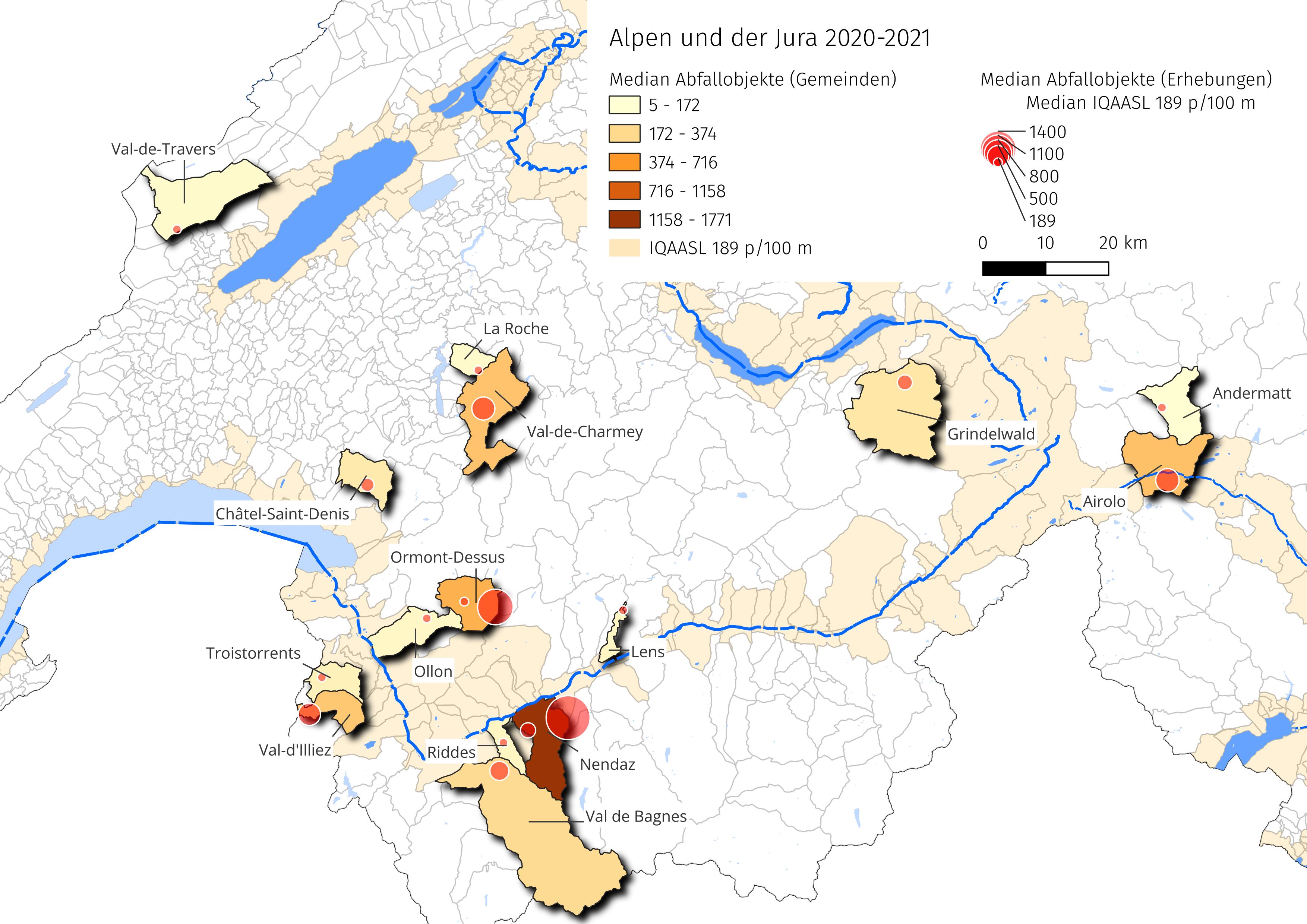
Abb. 2.1 #

Abbildung 2.1: Karte des Erhebungsgebiets Alpen und Jura, Clean-ups 2021.

Die Verantwortung für die Erhebungen in den Alpen und im Jura lag bei der Summit Foundation. Die Summit Foundation führt seit vielen Jahren Clean-ups (Gruppenevents, bei denen Müll aus dem Gelände beseitigt wird) in Schweizer Bergregionen durch. Zu den Clean-ups im Jahr 2021 gehörten auch eine Reihe von Erhebungen zu Abfallobjekten, die parallel zu den regelmässig stattfindenden Clean-ups durchgeführt wurden. Die Summit Foundation hatte zwei Fragen in Bezug auf IQAASL:

Wie kann die Datenerfassung in das aktuelle Geschäftsmodell integriert werden?
Was ergeben die Erhebungen auf den Bergpfaden im Vergleich zu denen am Wasser?

Der Zweck von Aufräumaktionen ist es, so viele Abfallobjekte wie möglich aus einem bestimmten Gebiet zu entfernen. Wie viel entfernt werden kann, hängt von den zur Verfügung stehenden Ressourcen ab. Eine Erhebung über Abfallobjekte dient der Identifizierung und Zählung der Objekte in einem bestimmten Gebiet. In diesem Sinne ist eine Aufräumaktion eine Annäherung an das Abfallproblem aus der Perspektive der Abschwächung oder Milderung, und Erhebungen liefern die notwendigen Daten zur Verbesserung der Prävention.

2.1. Erhebungsmethoden#

Insgesamt wurden zwanzig Erhebungen zu Abfallobjekten von der Summit Foundation durchgeführt. Ursprünglich wurden zwei Methoden ausgewählt:

Erhebungen entlang bestimmter Streckenabschnitte mit einer definierten Länge und Breite (inbesondere Wanderwege)
Erhebungen im Umfeld der Liftinfrastrukur (insbesondere Wartebereiche Schneesport)

Erhebungen im Umfeld der Liftinfrastrukur (insbesondere Wartebereiche Schneesport):

Ein Abschnitt des Weges oder der Fläche wird gemessen
Alle sichtbaren Verunreinigungen werden entfernt, gezählt und klassifiziert
Die Ergebnisse und Abmessungen werden aufgezeichnet

Der Unterschied zwischen den beiden Methoden liegt in der Art und Weise, wie die Grenzen des Vermessungsgebiets festgelegt werden. Wenn ein Weg benutzt wird, werden die Grenzen des Vermessungsgebiets durch den Weg selbst festgelegt, nicht durch die Person, die die Erhebung ausführt. Im Sommer sind die Barrieren und Schilder, welche Pisten etc. markieren, alle entfernt worden, so dass es für die Person, die die Erhebung ausführt, schwierig ist, die korrekten Grenzen genau zu bestimmen.

2.2. Kumulierte Gesamtzahlen für das Erhebungsgebiet#

Im Zeitraum von März 2020 bis Oktober 2021 wurden im Rahmen von 20 Datenerhebungen insgesamt 7 776 Objekte entfernt und identifiziert. Die Ergebnisse des Alpen und Jura umfassen 20 Orte, 18 Gemeinden und eine Gesamtbevölkerung von etwa 70 606 Einwohnenden.

Gemeinden

Airolo, Andermatt, Calanca, Châtel-Saint-Denis, Grindelwald, La Roche, Lens, Mesocco, Nendaz, Ollon, Ormont-Dessus, Riddes, Rovio, Troistorrents, Val de Bagnes, Val-d’Illiez, Val-de-Charmey, Val-de-Travers

2.2.1. Gesamtzahlen der Erhebungen#

Show code cell source Hide code cell source

# the dimensional sumaries for each trash count
dims_table = admin_details.dimensionalSummary()

# for this report columns need to be added to standard dimensions
# adding the pcs per unit column, add the region total first
dims_table.loc["Alpen und Jura", unit_label] = fdx.sample_totals[unit_label].median()

for location in admin_details.locations_of_interest:
    index_name = proper_names[location]
    value = unit_label_map.loc[location, unit_label]
    dims_table.loc[index_name, unit_label] = value

# !surprise! the surveyors used the micro plastics weight in  field to log the sample total weights in grams
# the total weight field was used to log the event total (in kilos), map these to the dims table
# which means the total weight column needs to be dropped from this view
new_columns = list(dims_table.columns)
new_columns.remove("total_w")
dims_table = dims_table[new_columns]

# map the mic_plas_w column back to the dims table
weights_map = admin_details.dims_data[["location", "mic_plas_w"]].set_index("location")

# add the cumulative total
dims_table.loc["Alpen und Jura", "Gesamtgewicht (Kg)"] = round(weights_map.mic_plas_w.sum()/1000, 2)


for location in admin_details.locations_of_interest:
    index_name = proper_names[location]
    value = weights_map.loc[location, "mic_plas_w"]
    dims_table.loc[index_name, "Gesamtgewicht (Kg)"] = round(value/1000, 2)

# format the table for display
# convert the plastic totals from grams to kilos
dims_table.mac_plast_w = (dims_table.mac_plast_w/1000).round(2)
dims_table = dims_table.sort_values(by="Gesamtgewicht (Kg)", ascending=False)

# convert samples, area, length and unit_label to integers
# the thousands are separated by a space not a comma or decimal
as_type_int = ["samples", "quantity", unit_label, "area", "length"]
dims_table[as_type_int] = dims_table[as_type_int].astype(int)

# rename the columns to german and reset the index
dims_table = dims_table.rename(columns=featuredata.dims_table_columns_de)
# dims_table.reset_index(inplace=True, drop=False)

dims_table.index.name = None
dims_table.columns.name = None

dims_table_formatter = {
    "Plastik (Kg)": lambda x: featuredata.replaceDecimal(x, "de"),
    "Gesamtgewicht (Kg)": lambda x: featuredata.replaceDecimal(x, "de"),
    "Fläche (m2)": lambda x: featuredata.thousandsSeparator(int(x), "de"),
    "Länge (m)": lambda x: featuredata.thousandsSeparator(int(x), "de"),
    "Erhebungen": lambda x: featuredata.thousandsSeparator(int(x), "de"),
    "Objekte (St.)": lambda x: featuredata.thousandsSeparator(int(x), "de")
    
    
}

# the columns of interest
alpes_columns = ["Gesamtgewicht (Kg)", "Plastik (Kg)", "Fläche (m2)", "Länge (m)", "Erhebungen", "Objekte (St.)"]
dims_table = dims_table[alpes_columns].copy()

# subsection title
subsection_title = Paragraph("Gesamtzahlen der Erhebungen", featuredata.subsection_title)

# a caption for the figure
dims_table_caption = 'Die aggregierten Ergebnisse der Abfallerhebungen. Ein Teil der Daten befindet sich aus Platzgründen in einer zweiten Tabelle darunter.'

q = dims_table.style.format(formatter=dims_table_formatter).set_table_styles(table_css_styles)
col_widths = [3.5*cm, 3*cm, *[2.2*cm]*(len(dims_table.columns)-1)]

# pdf table                 
d_chart = featuredata.aSingleStyledTable(dims_table, colWidths=col_widths)

table_caption = Paragraph(dims_table_caption, featuredata.caption_style)
table_and_caption = featuredata.tableAndCaption(d_chart, table_caption, col_widths)

new_components = [
    featuredata.large_space,
    subsection_title,
    featuredata.small_space,
    table_and_caption
]
pdfcomponents = featuredata.addToDoc(new_components, pdfcomponents)

glue(f'{this_feature["slug"]}_dims_table_caption', dims_table_caption, display=False)

glue(f'{this_feature["slug"]}_dims_table', q, display=False)

	Gesamtgewicht (Kg)	Plastik (Kg)	Fläche (m2)	Länge (m)	Erhebungen	Objekte (St.)
Alpen und Jura	18,85	6,35	6 856	1 237	20	7 776
La Tzoumaz	3,42	0,74	1 200	80	1	88
Andermatt	1,8	0,1	800	100	1	24
San Bernardino	1,56	0,8	11	5	1	431
Val Calanca	1,5	0,06	240	80	1	78
Robella	1,5	0,28	1 200	80	1	47
Nendaz	1,35	0,35	96	64	1	182
Tour Les Crosets	1,27	0,68	141	94	1	518
Les Diablerets	1,07	0,75	176	118	1	31
Cabanes des Diablerets	1,05	0,02	18	12	1	165
La Berra	1,01	0,01	1 500	60	1	34
Villars	0,63	0,3	550	110	1	105
Crans-Montana	0,56	0,36	64	43	1	47
Grindelwald	0,39	0,15	92	61	1	169
Verbier	0,37	0,16	74	50	1	205
Morgins	0,33	0,23	112	75	1	123
Charmey	0,33	0,91	150	30	1	174
Les Paccots	0,22	0,09	96	48	1	118
Airolo	0,2	0,14	57	38	1	224
Veysonnaz	0,15	0,12	164	12	1	4 981
Monte Generoso	0,14	0,1	115	77	1	32

Abb. 2.2 #

Abbildung 2.2: Die aggregierten Ergebnisse der Abfallerhebungen. Ein Teil der Daten befindet sich aus Platzgründen in einer zweiten Tabelle darunter.

2.2.2. Gesamtzahlen in Bezug auf die Clean-ups#

Show code cell source Hide code cell source

# the event totals include the amount collected but not counted
# the number of participants, the number of staff and the time to complete
event_totals = admin_details.dims_data[["location", "total_w", "num_parts_other", "num_parts_staff", "time_minutes"]].copy()

# the names are changed to proper names and set as the index
event_totals["location"] = event_totals.location.map(lambda x: proper_names.loc[x])
event_totals.set_index("location", inplace=True)

# sum all the events to give the total for the feauture
event_totals.loc[this_feature["name"]] = event_totals.sum(numeric_only=True, axis=0)

# convert minutes to hours
event_totals.time_minutes = (event_totals.time_minutes/60).round(1)
event_totals = event_totals.sort_values(by="total_w", ascending=False)

# formatting for display
thousands = ["total_w", "num_parts_other"]
event_totals[thousands] = event_totals[thousands].applymap(lambda x: featuredata.thousandsSeparator(int(x), "de"))
event_totals["time_minutes"] = event_totals.time_minutes.map(lambda x: featuredata.replaceDecimal(str(x)))

new_column_names = {
    "total_w":  "Gesamtgewicht (Kg)",
    "num_parts_other": "Teilnehmende", 
    "num_parts_staff": "Mitarbeitende",
    "time_minutes": "Std."
}

event_total_title = "Gesamtzahlen in Bezug auf die Clean-ups"
clean_up_subsection_title = Paragraph(event_total_title, featuredata.subsection_title)   

event_total_caption = [
    "Die Gesamtmenge des gesammelten Mülls in Kilogramm, die Anzahl ",
    "der Teilnehmenden und des Personals sowie die Zeit, die für die ",
    "Durchführung der Erhebung benötigt wurde."
]

event_caption = ''.join(event_total_caption)

table_two = event_totals.rename(columns=new_column_names)
col_widths=[3.5*cm, 3*cm, *[2.5*cm]*(len(table_two.columns)-2)]
table_two.index.name = None
table_two.columns.name = None

table_caption = Paragraph(event_caption, featuredata.caption_style)
d_chart = featuredata.aSingleStyledTable(table_two, colWidths=col_widths)
table_and_caption = featuredata.tableAndCaption(d_chart, table_caption, col_widths)
new_components = [
    featuredata.large_space,
    PageBreak(),
    clean_up_subsection_title,
    featuredata.small_space,
    table_and_caption,
    PageBreak()
]
pdfcomponents = featuredata.addToDoc(new_components, pdfcomponents)

q = table_two.style.set_table_styles(table_css_styles)

glue('event_summary_caption', event_caption, display=False)

glue('alpes_survey_area_event_summaries', q, display=False)

	Gesamtgewicht (Kg)	Teilnehmende	Mitarbeitende	Std.
Alpen und Jura	3 120	865	20	68,1
Cabanes des Diablerets	731	20	1	3,3
Andermatt	263	60	1	3,7
Villars	256	125	1	4,0
Charmey	235	72	1	3,7
Val Calanca	228	32	1	4,0
Tour Les Crosets	205	50	1	3,5
La Tzoumaz	200	50	1	4,0
Crans-Montana	185	35	1	2,5
Les Paccots	160	90	1	3,3
Nendaz	155	70	1	4,8
Morgins	129	60	1	4,0
La Berra	80	50	1	4,0
Verbier	76	27	1	2,0
Les Diablerets	74	40	1	3,0
Veysonnaz	48	12	1	4,0
Robella	37	23	1	3,3
Grindelwald	26	21	1	3,3
Monte Generoso	22	16	1	2,0
San Bernardino	9	12	1	4,0
Airolo	1	0	1	1,6

Abb. 2.3 #

Abbildung 2.3: Die Gesamtmenge des gesammelten Mülls in Kilogramm, die Anzahl der Teilnehmenden und des Personals sowie die Zeit, die für die Durchführung der Erhebung benötigt wurde.

2.2.3. Landnutzungsprofil der Erhebungsorte#

Das Landnutzungsprofil zeigt, welche Nutzungen innerhalb eines Radius von 1500 m um jeden Erhebungsort dominieren. Flächen werden einer von den folgenden vier Kategorien zugewiesen:

Fläche, die von Gebäuden eingenommen wird in %
Fläche, die dem Wald vorbehalten ist in %
Fläche, die für Aktivitäten im Freien genutzt wird in %
Fläche, die von der Landwirtschaft genutzt wird in %

Strassen (inkl. Wege) werden als Gesamtzahl der Strassenkilometer innerhalb eines Radius von 1500 m angegeben.

Es wird zudem angegeben, wie viele Flüsse innerhalb eines Radius von 1500 m um den Erhebungsort herum in das Gewässer münden.

Das Verhältnis der gefundenen Abfallobjekte unterscheidet sich je nach Landnutzungsprofil. Das Verhältnis gibt daher einen Hinweis auf die ökologischen und wirtschaftlichen Bedingungen um den Erhebungsort.

Für weitere Informationen siehe 17 Landnutzungsprofil

Show code cell source Hide code cell source

# this gets all the data for the project
land_use_kwargs = {
    "data": period_data.period_data,
    "index_column":"loc_date",
    "these_features": this_feature['slug'],
    "feature_level":this_feature['level']   
}

# the landuse profile of the project
project_profile = featuredata.LandUseProfile(**land_use_kwargs).byIndexColumn()

# update the kwargs for the feature data
land_use_kwargs.update({"data":fdx.feature_data})

# build the landuse profile of the feature
feature_profile = featuredata.LandUseProfile(**land_use_kwargs)

# this is the component features of the report
feature_landuse = feature_profile.featureOfInterest()

fig, axs = plt.subplots(2, 3, figsize=(9,8), sharey="row")

for i, n in enumerate(featuredata.default_land_use_columns):
    r = i%2
    c = i%3
    ax=axs[r,c]
    
    # the value of land use feature n
    # for each element of the feature
    for element in feature_landuse:
        # the land use data for a feature
        data = element[n].values
        # the name of the element
        element_name = element[feature_profile.feature_level].unique()
        # proper name for chart
        label = featuredata.river_basin_de[element_name[0]]
        # cumulative distribution        
        xs, ys = featuredata.empiricalCDF(data)
        # the plot of landuse n for this element
        sns.lineplot(x=xs, y=ys, ax=ax, label=label, color=featuredata.bassin_pallette[element_name[0]])
    
    # the value of the land use feature n for the project
    testx, testy = featuredata.empiricalCDF(project_profile[n].values)
    sns.lineplot(x=testx, y=testy, ax=ax, label=top, color="magenta")
    
    # get the median landuse for the feature
    the_median = np.median(data)
    
    # plot the median and drop horizontal and vertical lines
    ax.scatter([the_median], 0.5, color="red",s=40, linewidth=1, zorder=100, label="Median")
    ax.vlines(x=the_median, ymin=0, ymax=0.5, color="red", linewidth=1)
    ax.hlines(xmax=the_median, xmin=0, y=0.5, color="red", linewidth=1)
    
    if i <= 3:
        if c == 0:            
            ax.yaxis.set_major_locator(MultipleLocator(.1))
        ax.xaxis.set_major_formatter(ticker.PercentFormatter(1.0, 0, "%"))        
    else:
        pass      
    
    handles, labels = ax.get_legend_handles_labels()
    ax.get_legend().remove()    
    ax.set_title(featuredata.luse_de[n], loc='left')
    
plt.tight_layout()
plt.subplots_adjust(top=.91, hspace=.4)
plt.suptitle("Landnutzung im Umkries von 1 500 m um den Erhebungsort", ha="center", y=1, fontsize=16)
fig.legend(handles, labels, bbox_to_anchor=(.5,.5), loc="upper center", ncol=3)

figure_caption = [
    "Die Erhebungsorte in den Alpen und im Jura wiesen im Vergleich zu den Ergebungsorten IQAASL ",
    "einen höheren Prozentsatz an forst- und landwirtschaftlichen Flächen und einen geringeren ",
    "Prozentsatz an bebauter Fläche (Gebäude) und an Fläche, die für Aktivitäten im Freien genutzt werden, auf."
]

figure_caption = ''.join(figure_caption)
    
figure_name = f"{this_feature['slug']}_survey_area_landuse"
land_use_file_name = f'{save_fig_prefix}{figure_name}.jpeg'
save_figure_kwargs.update({"fname":land_use_file_name})

plt.tight_layout()
plt.subplots_adjust(top=.91, hspace=.4)
plt.savefig(**save_figure_kwargs)

# capture the output
glue(figure_name, fig, display=False)
glue("les-alpes_land_use_caption", figure_caption, display=False)
plt.close()

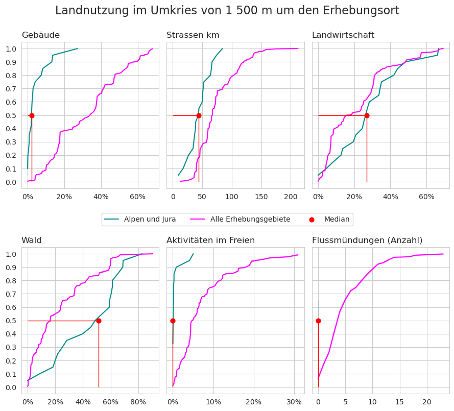
_images/0e8bafe962b21b80241e34a5b02c24c325c6720e8deec87617ccf7271f2174a6.png

Abb. 2.4 #

Abbildung 2.4: Die Erhebungsorte in den Alpen und im Jura wiesen im Vergleich zu den Ergebungsorten IQAASL einen höheren Prozentsatz an forst- und landwirtschaftlichen Flächen und einen geringeren Prozentsatz an bebauter Fläche (Gebäude) und an Fläche, die für Aktivitäten im Freien genutzt werden, auf.

Die aggregierten Ergebnisse zeigen den Unterschied zwischen den beiden Erhebungsmethoden. Die drei Erhebungsorte mit dem höchsten p/100 m haben auch die kürzeste Länge. Im Fall von Cabanes-des-Diablerets entspricht die Fläche (in m2) der Länge (in m), was darauf hindeutet, dass ein kleiner Bereich um eine Struktur oder ein Gebäude herum vermessen wurde. In Veysonnaz befindet sich die Talstation der Seilbahn nach Thyon (Wintersportgebiet Veysonnaz / 4 Vallées).

Der Unterschied in den Methoden führt zu abweichenden Ergebnissen. Ausserdem wurden diese beiden Orte aufgrund der früheren Erfahrungen der Person, die die Erhebung ausführt, speziell für die Bestandsaufnahme ausgewählt. Wegen der unterschiedlichen Dimensionen und Methoden werden die Erhebungsergebnisse aus Veysonnaz, San-Beranardino und Cabanes-des-Diablerets in der weiteren Analyse nicht berücksichtigt.

2.3. Verteilung der Erhebungsergebnisse¶#

Show code cell source Hide code cell source

dx = period_data.parentSampleTotals(parent=False)

not_trail_samples = ["veysonnaz", "cabanes-des-diablerets", "san-bernardino"]

fdt = fd[~fd.location.isin(not_trail_samples)].copy()
fdt_samples = fdx.sample_totals[~fdx.sample_totals.location.isin(not_trail_samples)].copy()

material_map = fdx.mMap
description_map = fdx.dMap

fig, axs = plt.subplots(1,2, figsize=(10,5))

months = mdates.MonthLocator(interval=1)
months_fmt = mdates.DateFormatter("%b")
days = mdates.DayLocator(interval=7)

ax = axs[0]
ax.set_ylim(-50, 2000)

# the cumlative distributions:
axtwo = axs[1]

# feature surveys
sns.scatterplot(data=dx, x="date", y=unit_label, label=top, color="black", alpha=0.3,  ax=ax)
# all other surveys
sns.scatterplot(data=fdt_samples, x="date", y=unit_label, label=this_feature["name"], color=bassin_pallette[this_feature["slug"]], edgecolor="white", ax=ax)

ax.set_ylabel(unit_label, **ck.xlab_k14)
ax.set_xlabel("")
ax.xaxis.set_minor_locator(days)
ax.xaxis.set_major_formatter(months_fmt)

axtwo = axs[1]

box_props = {
    "boxprops":{"facecolor":"none", "edgecolor":"magenta"},
    "medianprops":{"color":"magenta"},
    "whiskerprops":{"color":"magenta"},
    "capprops":{"color":"magenta"}
}
sns.boxplot(data=dx, y=unit_label, color="black",  ax=axtwo, showfliers=False, **box_props, zorder=1)
sns.stripplot(data=dx[dx[unit_label] <= 1000], s=10, y=unit_label, color="black", ax=axtwo, alpha=0.5, jitter=0.3, zorder=0)
sns.stripplot(data=fdt_samples[fdt_samples[unit_label] <= 1000], y=unit_label, color=bassin_pallette[this_feature["slug"]], s=10, edgecolor="white",linewidth=1, ax=axtwo, jitter=0.3, zorder=2)

axtwo.set_xlabel("")
axtwo.set_ylabel(unit_label, **ck.xlab_k14)
axtwo.tick_params(which="both", axis="x", bottom=False)
ax.legend()

plt.tight_layout()

figure_name = f"{this_feature['slug']}_sample_totals"
sample_totals_file_name = f'{save_fig_prefix}{figure_name}.jpeg'
save_figure_kwargs.update({"fname":sample_totals_file_name})
plt.savefig(**save_figure_kwargs)

# figure caption
sample_total_notes = [
    "Links: Zusammenfassung der Daten aller Erhebungen Erhebungsgebiet Alpes März 2020 bis September 2021, n=20. ",
    "Rechts: Gefundene Materialarten im Erhebungsgebiet Alpes in Stückzahlen und als prozentuale Anteile (stückzahlbezogen). ",
]

sample_total_notes = ''.join(sample_total_notes)

glue(f'{this_feature["slug"]}_sample_total_notes', sample_total_notes, display=False)

glue(f'{this_feature["slug"]}_sample_totals', fig, display=False)
plt.close()

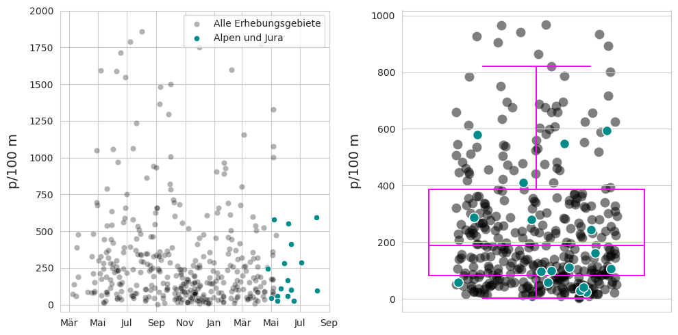
_images/a307ea8121c4c83edc6a870771fee2082540a620742e710415566d60973d5214.png

Abb. 2.5 #

Abbildung 2.5: Links: Zusammenfassung der Daten aller Erhebungen Erhebungsgebiet Alpes März 2020 bis September 2021, n=20. Rechts: Gefundene Materialarten im Erhebungsgebiet Alpes in Stückzahlen und als prozentuale Anteile (stückzahlbezogen).

2.3.1. Zusammenfassende Daten und Materialtypen#

Show code cell source Hide code cell source

def columnsAndOperations(column_operations: list = None, columns: list = None, unit_label: str = None):
    if column_operations is None:
        column_operation = {unit_label: "median", "quantity": "sum"}
    else:
        column_operation = {x[0]: x[1] for x in column_operations}
    if columns is None:
        columns = ["loc_date", "groupname"]
    
    return columns, column_operation

def changeSeriesIndexLabels(a_series: pd.Series = None, change_names: {} = None):
    """A convenience function to change the index labels of a series x.
    Change_names is keyed to the series index.

    :param a_series: A pandas series
    :param change_names: A dictionary that has keys = x.index and values = new x.index label
    :return: The series with the new labels
    """
    
    new_dict = {}
    for param in a_series.index:
        new_dict.update({change_names[param]: a_series[param]})
    return pd.Series(new_dict)

def createSummaryTableIndex(unit_label, language="en"):
    """Assigns the current units to the keys and creates
    custom key values based on language selection.

    :param unit_label: The current value of unit label
    :param language: the two letter abbreviation for the current language
    :return: the pd.describe dict with custom labels
    """
    
    if language == "en":
        new_data = {"count": "# samples",
                    "mean": f"average {unit_label}",
                    "std": "standard deviation",
                    "min": f"min {unit_label}",
                    "max": f"max {unit_label}",
                    "25%": "25%",
                    "50%": "50%",
                    "75%": "75%",
                    "total objects": "total objects",
                    "# locations": "# locations",
                    }
    elif language == "de":
        new_data = {"count": "Erhebungen",
                    "mean": f"Durchschnitt {unit_label}",
                    "std": "Standardabweichung",
                    "min": f"min {unit_label}",
                    "max": f"max {unit_label}",
                    "25%": "25%",
                    "50%": "50%",
                    "75%": "75%",
                    "total objects": "Abfallobjekte",
                    "# locations": "Anzahl der Standorte",
                    }
    else:
        print(f"ERROR {language} is not an option")
        new_data = {}
    
    return new_data

def makeDailyTotalSummary(
    sample_totals: pd.DataFrame = None, unit_label: str = None, language: str = None):

    # the summary of the dependent variable
    a = sample_totals[unit_label].describe().round(2)
    a["total objects"] = sample_totals.quantity.sum()

    # assign appropriate language to index names
    # retrieve the appropriate index names based on language
    table_index = createSummaryTableIndex(unit_label, language=language)

    # assign the new index
    summary_table = changeSeriesIndexLabels(a, table_index)

    return summary_table

def codeSummary(
    feature_data: pd.DataFrame = None, unit_label: str = None, column_operations=None,
    material_map: pd.DataFrame = None, description_map: pd.DataFrame = None):

        
    if column_operations is None:
        column_operations = {
            "column_operations": [(unit_label, "median"), ("quantity", "sum")],
            "columns": ["code"],
            "unit_label": unit_label
        }

    columns, column_operation = columnsAndOperations(**column_operations)

    # apply the column operations
    code_totals = feature_data.groupby(columns, as_index=False).agg(column_operation)
    # percent of total
    code_totals["% of total"] = ((code_totals.quantity / code_totals.quantity.sum()) * 100).round(2)
    # fail and fail-rate
    code_totals["fail"] = code_totals.code.map(lambda x: feature_data[
        (feature_data.code == x) & (feature_data.quantity > 0)].loc_date.nunique())
    
    code_totals["fail rate"] = ((code_totals.fail / feature_data.loc_date.nunique()) * 100).astype("int")

    # the code data comes from the feature data (survey results)
    # Add the description of the code and the material
    code_totals.set_index(columns, inplace=True)
    code_totals["item"] = code_totals.index.map(lambda x: description_map[x])
    code_totals["material"] = code_totals.index.map(lambda x: material_map[x])

    code_totals = code_totals[["item", "quantity", "% of total", unit_label, "fail rate", "material"]]

    return code_totals

def materialSummary(code_summary: pd.DataFrame = None):
    a = code_summary.groupby("material", as_index=False).quantity.sum()
    a["% of total"] = a['quantity'] / a['quantity'].sum()
    b = a.sort_values(by="quantity", ascending=False)
    
    return b

def mostCommon(code_summary: pd.DataFrame = None, fail_rate: int = None, limit: int = 10):
    # the top ten by quantity
    most_abundant = code_summary.sort_values(by="quantity", ascending=False)[:limit]
    # the most common
    most_common = code_summary[code_summary["fail rate"] >= fail_rate].sort_values(by="quantity", ascending=False)
    # merge with most_common and drop duplicates
    # it is possible (likely) that a code will be abundant and common
    m_common = pd.concat([most_abundant, most_common]).drop_duplicates()

    return m_common

s_table_kwargs = {
    "sample_totals": fdt_samples,
    "unit_label": unit_label,
    "language": language
}

code_summary_kwargs = {
    "feature_data": fdt,
    "unit_label": unit_label,
    "column_operations": None,
    "description_map": description_map,
    "material_map": material_map
}


code_summary = codeSummary(**code_summary_kwargs)
cs = makeDailyTotalSummary(**s_table_kwargs)

combined_summary =[(x, featuredata.thousandsSeparator(int(cs[x]), language)) for x in cs.index]


# the materials table
fd_mat_totals = materialSummary(code_summary=code_summary)
fd_mat_totals = featuredata.fmtPctOfTotal(fd_mat_totals, around=0)

# applly new column names for printing
cols_to_use = {"material":"Material","quantity":"Objekte (St.)", "% of total":"Anteil"}
fd_mat_t = fd_mat_totals[cols_to_use.keys()].values
fd_mat_t = [(x[0], featuredata.thousandsSeparator(int(x[1]), language), x[2]) for x in fd_mat_t]

# make tables
fig, axs = plt.subplots(1,2)

# names for the table columns
a_col = [this_feature["name"], "Total"]

axone = axs[0]
sut.hide_spines_ticks_grids(axone)

table_two = sut.make_a_table(axone, combined_summary,  colLabels=a_col, colWidths=[.75,.25],  bbox=[0,0,1,1], **{"loc":"lower center"})
table_two.get_celld()[(0,0)].get_text().set_text(" ")
table_two.set_fontsize(12)

# material table
axtwo = axs[1]
axtwo.set_xlabel(" ")
sut.hide_spines_ticks_grids(axtwo)

table_three = sut.make_a_table(axtwo, fd_mat_t,  colLabels=list(cols_to_use.values()), colWidths=[.4, .4,.2],  bbox=[0,0,1,1], **{"loc":"lower center"})
table_three.get_celld()[(0,0)].get_text().set_text(" ")
table_three.set_fontsize(12)
plt.tight_layout()
plt.subplots_adjust(wspace=0.1)
# figure caption
summary_of_survey_totals = [
    "Links: Zusammenfassung der erhebungen entlang der Wanderwege. ",
    "Rechts: Aufschlüsselung nach Materialart (Stückzahlen und prozentuale Verteilung)."
]

summary_of_survey_totals = ''.join(summary_of_survey_totals)
glue(f'{this_feature["slug"]}_sample_summaries_caption', summary_of_survey_totals, display=False)

figure_name = f'{this_feature["slug"]}_sample_summaries'
sample_summaries_file_name = f'{save_fig_prefix}{figure_name}.jpeg'
save_figure_kwargs.update({"fname":sample_summaries_file_name})

plt.savefig(**save_figure_kwargs)
glue('les-alpes_sample_material_tables', fig, display=False)
plt.close()

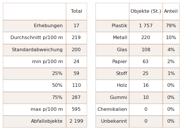
_images/ea0eba375e5ba849709455c3a32a38706a8f83932d6fa7961172d89a103758d5.png

Abb. 2.6 #

Abbildung 2.6: Links: Zusammenfassung der erhebungen entlang der Wanderwege. Rechts: Aufschlüsselung nach Materialart (Stückzahlen und prozentuale Verteilung).

2.4. Die am häufigsten gefundenen Objekte#

Die am häufigsten gefundenen Objekte sind die zehn mengenmässig am meisten vorkommenden Objekte und/oder Objekte, die in mindestens 50 % aller Erhebungen identifiziert wurden (Häufigkeitsrate).

	Objekte (St.)	Anteil	Häufigkeitsrate	p/100 m
Seilbahnbürsten	461	20%	5%	0,0
Zigarettenfilter	270	12%	94%	11,0
Fragmentierte Kunststoffe	222	10%	100%	12,0
Snack-Verpackungen	187	8%	100%	11,0
Schrauben und Bolzen	81	3%	64%	3,0
Kabelbinder	73	3%	64%	2,0
Getränkeflaschen aus Glas, Glasfragmente	67	3%	41%	0,0
Verpackungen aus Aluminiumfolie	67	3%	64%	2,0
Andere Kunststoff	60	2%	5%	0,0
Abdeckklebeband/Verpackungsklebeband	48	2%	64%	3,0

Abb. 2.7 #

Abbildung 2.7: Häufigste Objekte auf Wanderwegen: Objekte mit einer Häufigkeitsrate von mindestens 50 % und/oder die 10 häufigsten Objekte. Zusammengenommen stellen die zehn häufigsten Objekte 69 % aller gefundenen Objekte dar. p/100 m: Medianwert der Erhebung.

2.4.1. Die am häufigsten gefundenen Gegenstände nach Erhebungsort#

Show code cell source Hide code cell source

def componentMostCommonPcsM(
    feature_data: pd.DataFrame = None, most_common: pd.DataFrame = None, columns: list = None, unit_label: str = None,
    feature_component: str = None, column_operations: list = None, description_map: pd.DataFrame = None):

    codes = most_common.index
    
    if column_operations is None:        
        column_operations = {
            "column_operations":  [(unit_label, "sum"), ("quantity", "sum")],
            "columns":  [feature_component, "loc_date", "code"],
            "unit_label": unit_label
        }

    columns, column_operation = columnsAndOperations(**column_operations)

    mask = feature_data.code.isin(codes)    

    a = feature_data[mask].groupby(columns, as_index=False).agg(column_operation)
    a = a.groupby([feature_component, "code"], as_index=False)[unit_label].median()

    # map the description to the code
    a["item"] = a.code.map(lambda x: description_map.loc[x])

    return a

       
def parentMostCommon(parent_data: pd.DataFrame = None, most_common: list = None, unit_label: str = None, 
                     percent: bool = False, name: str = None):
    
    data = parent_data[parent_data.code.isin(most_common)]   

    if percent:
        data = data.groupby('code', as_index=False).quantity.sum()
        data.set_index('code', inplace=True)
        data[name] = (data.quantity / data.quantity.sum()).round(2)

        return data[name]

    else:
        data = data.groupby(["loc_date", 'code'], as_index=False)[unit_label].sum()
        data = data.groupby('code', as_index=False)[unit_label].median()
        data.set_index('code', inplace=True)
        data[name] = data[unit_label]

        return data[name]
    
aggregate_kwargs = {
    "parent_data": period_data.period_data,
    "most_common": mcc.index,
    "unit_label": unit_label,
    "percent": False,
    "name":"IQAASL",
}

component_kwargs = {
    "feature_data": fdt,
    "most_common": most_common,
    "feature_component": fdx.feature_component,
    "unit_label": unit_label,
    "description_map": description_map,
}
    
# the columns needed to build the heat map
heat_map_columns = ["item", "location", unit_label]

# the results for the most common codes at the component level
components = componentMostCommonPcsM(**component_kwargs)

# pivot that to make a heat map layouy
mc_comp = components[heat_map_columns].pivot(columns='location', index='item')

# drop any indexing above the component name
mc_comp.columns = mc_comp.columns.get_level_values(1)
mc_comp.rename(columns={x:proper_names[x] for x in mc_comp.columns}, inplace=True)

# switch the index to the item description
mc_feature = mcc[["item", unit_label]].set_index("item")

# add a column for the results of all the feature data
mc_comp[this_feature["name"]] = mc_feature

# get the resluts of the feature most common from IQAASL results
iqaasl_results = parentMostCommon(**aggregate_kwargs)

# replace the code with a description
new_labels = {x : description_map[x] for x in iqaasl_results.index}
mc_iqaasl = featuredata.changeSeriesIndexLabels(a_series=iqaasl_results, change_names=new_labels)

# add a column for the results of all the IQAASL data
mc_comp["IQAASL"] = mc_iqaasl

caption_prefix =  f"Verwendungszweck der gefundenen Objekte an Wanderwegen: Median {unit_label} am "
col_widths=[4.5*cm, *[1.2*cm]*(len(mc_comp.columns)-1)]
mc_heatmap_title = Paragraph("Die am häufigsten gefundenen Gegenstände nach Erhebungsort", featuredata.subsection_title)
mc_heat_map_caption = "Verwendungszweck der gefundenen Objekte an Wanderwegen: Median p/100 m."
tables = featuredata.splitTableWidth(mc_comp, gradient=True, caption_prefix=caption_prefix, caption=mc_heat_map_caption,
                    this_feature=this_feature["name"], vertical_header=True, colWidths=col_widths)

# identify the tables variable as either a list or a Flowable:
if isinstance(tables, (list, np.ndarray)):
    grouped_pdf_components = [mc_heatmap_title, featuredata.large_space, *tables]
else:
    grouped_pdf_components = [mc_heatmap_title, featuredata.large_space, tables]    

new_components = [
    smallspace,
    *grouped_pdf_components
]

pdfcomponents = featuredata.addToDoc(new_components, pdfcomponents)

aformatter = {x: featuredata.replaceDecimal for x in mc_comp.columns}
mcd = mc_comp.style.format(aformatter).set_table_styles(heat_map_css_styles)
mcd = mcd.background_gradient(axis=None, vmin=mc_comp.min().min(), vmax=mc_comp.max().max(), cmap="YlOrBr")
mcd = mcd.applymap_index(featuredata.rotateText, axis=1)
mcd.index.name = None
mcd.columns.name = None
glue('alpes_survey_area_most_common_heat_map', mcd, display=False)

	Airolo	Andermatt	Charmey	Crans-Montana	Grindelwald	La Berra	Robella	La Tzoumaz	Tour Les Crosets	Les Diablerets	Les Paccots	Monte Generoso	Morgins	Nendaz	Val Calanca	Verbier	Villars	Alpen und Jura	IQAASL
Getränkeflaschen aus Glas, Glasfragmente	34,0	2,0	0,0	0,0	0,0	3,0	31,0	3,0	0,0	0,0	2,0	0,0	0,0	0,0	28,0	0,0	0,0	0,0	3,0
Abdeckklebeband/Verpackungsklebeband	21,0	1,0	17,0	5,0	0,0	0,0	1,0	10,0	0,0	0,0	12,0	0,0	3,0	12,0	0,0	8,0	3,0	3,0	0,0
Andere Kunststoff	0,0	0,0	0,0	0,0	0,0	0,0	0,0	0,0	0,0	0,0	0,0	0,0	0,0	94,0	0,0	0,0	0,0	0,0	0,0
Fragmentierte Kunststoffe	69,0	3,0	147,0	7,0	12,0	12,0	1,0	22,0	1,0	3,0	67,0	4,0	49,0	23,0	5,0	28,0	4,0	12,0	18,0
Kabelbinder	8,0	0,0	37,0	2,0	2,0	0,0	0,0	0,0	0,0	2,0	29,0	3,0	7,0	45,0	0,0	8,0	1,0	2,0	0,0
Schrauben und Bolzen	3,0	0,0	7,0	9,0	3,0	0,0	0,0	0,0	12,0	0,0	25,0	0,0	12,0	25,0	3,0	42,0	1,0	3,0	0,0
Seilbahnbürsten	0,0	0,0	0,0	0,0	0,0	0,0	0,0	0,0	490,0	0,0	0,0	0,0	0,0	0,0	0,0	0,0	0,0	0,0	0,0
Snack-Verpackungen	84,0	1,0	63,0	9,0	72,0	15,0	3,0	11,0	6,0	2,0	12,0	3,0	17,0	27,0	1,0	24,0	7,0	11,0	9,0
Verpackungen aus Aluminiumfolie	74,0	0,0	27,0	0,0	15,0	3,0	0,0	4,0	0,0	2,0	10,0	3,0	1,0	0,0	0,0	12,0	1,0	2,0	0,0
Zigarettenfilter	66,0	3,0	50,0	16,0	125,0	2,0	5,0	9,0	0,0	2,0	12,0	3,0	24,0	3,0	17,0	152,0	11,0	11,0	20,0

Abb. 2.8 #

Abbildung 2.8: Häufigste Objekte an Wanderwegen: Median p/100 m.

2.4.2. Seilbahnbürsten#

Abb. 2.9 #

Abbildung 2.9: Seilbahnbürsten, die verwendet werden, um Eis und Schnee von Skiliften zu entfernen, können sich von der Anlage lösen und Tausende von schweren Kunststofffäden erzeugen.

2.5. Verwendungszweck der gefundenen Objekte#

Der Verwendungszweck basiert auf der Verwendung des Objekts, bevor es weggeworfen wurde, oder auf der Artikelbeschreibung, wenn die ursprüngliche Verwendung unbestimmt ist. Identifizierte Objekte werden einer der 260 vordefinierten Kategorien zugeordnet. Die Kategorien werden je nach Verwendung oder Artikelbeschreibung gruppiert.

Abwasser: Objekte, die aus Kläranlagen freigesetzt werden, sprich Objekte, die wahrscheinlich über die Toilette entsorgt werden
Mikroplastik (< 5 mm): fragmentierte Kunststoffe und Kunststoffharze aus der Vorproduktion
Infrastruktur: Artikel im Zusammenhang mit dem Bau und der Instandhaltung von Gebäuden, Strassen und der Wasser-/Stromversorgung
Essen und Trinken: alle Materialien, die mit dem Konsum von Essen und Trinken in Zusammenhang stehen
Landwirtschaft: Materialien z. B. für Mulch und Reihenabdeckungen, Gewächshäuser, Bodenbegasung, Ballenverpackungen. Einschliesslich Hartkunststoffe für landwirtschaftliche Zäune, Blumentöpfe usw.
Tabakwaren: hauptsächlich Zigarettenfilter, einschliesslich aller mit dem Rauchen verbundenen Materialien
Freizeit und Erholung: Objekte, die mit Sport und Freizeit zu tun haben, z. B. Angeln, Jagen, Wandern usw.
Verpackungen ausser Lebensmittel und Tabak: Verpackungsmaterial, das nicht lebensmittel- oder tabakbezogen ist
Plastikfragmente: Plastikteile unbestimmter Herkunft oder Verwendung
Persönliche Gegenstände: Accessoires, Hygieneartikel und Kleidung

Im Anhang (Kapitel 3.6.3) befindet sich die vollständige Liste der identifizierten Objekte, einschliesslich Beschreibungen und Gruppenklassifizierung. Das Kapitel 16 Codegruppen beschreibt jede Codegruppe im Detail und bietet eine umfassende Liste aller Objekte in einer Gruppe.

Unten: Wanderwege Nutzen der gefundenen Objekte: % der Gesamtzahl nach Wassermerkmal. Fragmentierte Objekte, die nicht eindeutig identifiziert werden können, bleiben nach Grösse klassifiziert.

Show code cell source Hide code cell source

def parentGroupTotals(data: pd.DataFrame = None, most_common: list = None, unit_label: str = None, 
                     percent: bool = False, name: str = None):
    
    if percent:
        data = data.groupby('groupname', as_index=False).quantity.sum()
        data.set_index('groupname', inplace=True)
        data[name] = (data.quantity / data.quantity.sum()).round(2)

        return data[name]

    else:
        data = data.groupby(["loc_date", 'groupname'], as_index=False)[unit_label].sum()
        data = data.groupby('groupname', as_index=False)[unit_label].median()
        data.set_index('groupname', inplace=True)
        data[name] = data[unit_label]

        return data[name]



# the results are a callable for the components
components = fdx.componentCodeGroupResults()
pt_comp = components[~components.location.isin(not_trail_samples)][["location", "groupname", '% of total' ]].pivot(columns="location", index="groupname")

# pivot that and reomve any hierarchal column index
pt_comp.columns = pt_comp.columns.get_level_values(1)
pt_comp.rename(columns = {x:proper_names[x] for x in pt_comp.columns}, inplace=True)

aggregate_kwargs = {
    "data": period_data.period_data,
    "unit_label": unit_label,
    "percent": True,
    "name":"IQAASL",
}        

    
component_kwargs = {
    "data":fdt,    
    "unit_label": unit_label,
    "name": this_feature["name"],
    "percent": True
    
}

pt_comp[this_feature["name"]] = parentGroupTotals(**component_kwargs)
pt_comp["IQAASL"] = parentGroupTotals(**aggregate_kwargs)

# pdf out put

caption_prefix =  f"Verwendungszweck der gefundenen Objekte an Wanderwegen: "
col_widths=[4.5*cm, *[1.2*cm]*(len(mc_comp.columns)-1)]
codegroup_heatmap_title = [
    "Unten: Wanderwege Nutzen der gefundenen Objekte: % der Gesamtzahl nach Wassermerkmal. Fragmentierte Objekte, ",
    "die nicht eindeutig identifiziert werden können, bleiben nach Grösse klassifiziert."
]

codegroup_heatmap_title = ''.join(codegroup_heatmap_title)
table_title = Paragraph(codegroup_heatmap_title, featuredata.p_style)

mc_heat_map_caption = "Verwendungszweck der gefundenen Objekte an Wanderwegen: Median p/100 m."
tables = featuredata.splitTableWidth(pt_comp, gradient=True, caption_prefix=caption_prefix, caption=mc_heat_map_caption,
                                     this_feature=this_feature["name"], vertical_header=True, colWidths=col_widths)

# identify the tables variable as either a list or a Flowable:
if isinstance(tables, (list, np.ndarray)):
    grouped_pdf_components = [table_title, featuredata.small_space, *tables]
else:
    grouped_pdf_components = [table_title, featuredata.small_space, tables]
    

new_components = [
    smallspace,
    *grouped_pdf_components
]

pdfcomponents = featuredata.addToDoc(new_components, pdfcomponents)
pt_comp.index.name = None
pt_comp.columns.name = None
aformatter = {x: '{:.0%}' for x in pt_comp.columns}

ptd = pt_comp.style.format(aformatter).set_table_styles(heat_map_css_styles).background_gradient(axis=None, vmin=pt_comp.min().min(), vmax=pt_comp.max().max(), cmap="YlOrBr")
ptd = ptd.applymap_index(featuredata.rotateText, axis=1)
glue('alpes_survey_area_codegroup_percent', ptd, display=True)

	Airolo	Andermatt	Charmey	Crans-Montana	Grindelwald	La Berra	Robella	La Tzoumaz	Tour Les Crosets	Les Diablerets	Les Paccots	Monte Generoso	Morgins	Nendaz	Val Calanca	Verbier	Villars	Alpen und Jura	IQAASL
Abwasser	0%	0%	1%	0%	1%	0%	0%	1%	0%	0%	0%	0%	2%	0%	0%	0%	0%	0%	5%
Essen und Trinken	50%	29%	16%	23%	34%	41%	70%	19%	3%	19%	12%	22%	16%	13%	33%	16%	21%	20%	19%
Freizeit und Erholung	4%	0%	3%	11%	2%	9%	2%	7%	1%	0%	3%	0%	9%	1%	3%	3%	6%	3%	4%
Infrastruktur	7%	21%	24%	21%	2%	9%	9%	33%	91%	39%	44%	38%	16%	32%	29%	14%	6%	36%	18%
Landwirtschaft	0%	4%	1%	2%	0%	0%	0%	2%	0%	26%	2%	25%	1%	0%	3%	0%	3%	1%	6%
Mikroplastik (< 5mm)	4%	0%	0%	9%	8%	0%	0%	0%	0%	0%	0%	0%	0%	1%	0%	3%	0%	2%	8%
Persönliche Gegenstände	4%	8%	8%	6%	1%	18%	2%	6%	3%	0%	1%	0%	4%	3%	4%	0%	45%	5%	3%
Plastikfragmente	12%	12%	25%	6%	4%	21%	2%	20%	0%	10%	27%	9%	30%	8%	5%	7%	4%	10%	14%
Tabakwaren	12%	12%	11%	17%	47%	3%	9%	9%	0%	6%	7%	6%	15%	2%	18%	37%	12%	13%	17%
Verpackungen ohne Lebensmittel/Tabak	5%	4%	7%	2%	0%	0%	6%	2%	1%	0%	4%	0%	7%	6%	5%	16%	4%	5%	5%
nicht klassifiziert	0%	8%	5%	2%	1%	0%	0%	0%	0%	0%	0%	0%	0%	34%	0%	3%	0%	4%	1%

	Airolo	Andermatt	Charmey	Crans-Montana	Grindelwald	La Berra	Robella	La Tzoumaz	Tour Les Crosets	Les Diablerets	Les Paccots	Monte Generoso	Morgins	Nendaz	Val Calanca	Verbier	Villars	Alpen und Jura	IQAASL
Abwasser	0%	0%	1%	0%	1%	0%	0%	1%	0%	0%	0%	0%	2%	0%	0%	0%	0%	0%	5%
Essen und Trinken	50%	29%	16%	23%	34%	41%	70%	19%	3%	19%	12%	22%	16%	13%	33%	16%	21%	20%	19%
Freizeit und Erholung	4%	0%	3%	11%	2%	9%	2%	7%	1%	0%	3%	0%	9%	1%	3%	3%	6%	3%	4%
Infrastruktur	7%	21%	24%	21%	2%	9%	9%	33%	91%	39%	44%	38%	16%	32%	29%	14%	6%	36%	18%
Landwirtschaft	0%	4%	1%	2%	0%	0%	0%	2%	0%	26%	2%	25%	1%	0%	3%	0%	3%	1%	6%
Mikroplastik (< 5mm)	4%	0%	0%	9%	8%	0%	0%	0%	0%	0%	0%	0%	0%	1%	0%	3%	0%	2%	8%
Persönliche Gegenstände	4%	8%	8%	6%	1%	18%	2%	6%	3%	0%	1%	0%	4%	3%	4%	0%	45%	5%	3%
Plastikfragmente	12%	12%	25%	6%	4%	21%	2%	20%	0%	10%	27%	9%	30%	8%	5%	7%	4%	10%	14%
Tabakwaren	12%	12%	11%	17%	47%	3%	9%	9%	0%	6%	7%	6%	15%	2%	18%	37%	12%	13%	17%
Verpackungen ohne Lebensmittel/Tabak	5%	4%	7%	2%	0%	0%	6%	2%	1%	0%	4%	0%	7%	6%	5%	16%	4%	5%	5%
nicht klassifiziert	0%	8%	5%	2%	1%	0%	0%	0%	0%	0%	0%	0%	0%	34%	0%	3%	0%	4%	1%

Abb. 2.10 #

Abbildung 2.10: Verwendungszweck der gefundenen Objekte an Wanderwegen: prozentualer Anteil an der Gesamtzahl nach Verwendungszweck. Fragmentierte Objekte, die nicht eindeutig identifiziert werden können, bleiben nach Grösse klassifiziert.

Show code cell source Hide code cell source

aggregate_kwargs = {
    "data": period_data.period_data,
    "unit_label": unit_label,
    "percent": False,
    "name":"IQAASL",
}        

pt_comp =  components[~components.location.isin(not_trail_samples)][["location", "groupname", unit_label]].pivot(columns="location", index="groupname")

# quash the hierarchal column index
pt_comp.columns = pt_comp.columns.get_level_values(1)
pt_comp.rename(columns = {x:proper_names[x] for x in pt_comp.columns}, inplace=True)
pt_comp[this_feature["name"]] = parentGroupTotals(**component_kwargs)
pt_comp["IQAASL"] = parentGroupTotals(**aggregate_kwargs)

caption_prefix =  f"Verwendungszweck der gefundenen Objekte an Wanderwegen: "
col_widths=[4.5*cm, *[1.2*cm]*(len(mc_comp.columns)-1)]
codegroup_heatmap_title = [
    f"Unten: Wanderwege Nutzen der gefundenen Objekte: {unit_label} der Gesamtzahl nach Wassermerkmal. Fragmentierte Objekte, ",
    "die nicht eindeutig identifiziert werden können, bleiben nach Grösse klassifiziert."
]

codegroup_heatmap_title = ''.join(codegroup_heatmap_title)
table_title = Paragraph(codegroup_heatmap_title, featuredata.p_style)

mc_heat_map_caption = "Verwendungszweck der gefundenen Objekte an Wanderwegen: Median p/100 m."
tables = featuredata.splitTableWidth(pt_comp, gradient=True, caption_prefix=caption_prefix, caption=mc_heat_map_caption,
                    this_feature=this_feature["name"], vertical_header=True, colWidths=col_widths)

# identify the tables variable as either a list or a Flowable:
if isinstance(tables, (list, np.ndarray)):
    grouped_pdf_components = [table_title, featuredata.small_space, *tables]
else:
    grouped_pdf_components = [table_title, featuredata.small_space, tables]
    

new_components = [
    smallspace,
    *grouped_pdf_components
]

pdfcomponents = featuredata.addToDoc(new_components, pdfcomponents)

# format for display
pt_comp.index.name = None
pt_comp.columns.name = None
aformatter = {x: featuredata.replaceDecimal for x in pt_comp.columns}
ptd = pt_comp.style.format(aformatter).set_table_styles(heat_map_css_styles).background_gradient(axis=None, vmin=pt_comp.min().min(), vmax=pt_comp.max().max(), cmap="YlOrBr")
ptd = ptd.applymap_index(featuredata.rotateText, axis=1)
glue('alpes_survey_area_codegroup_pcsm', ptd, display=False)

	Airolo	Andermatt	Charmey	Crans-Montana	Grindelwald	La Berra	Robella	La Tzoumaz	Tour Les Crosets	Les Diablerets	Les Paccots	Monte Generoso	Morgins	Nendaz	Val Calanca	Verbier	Villars	Alpen und Jura	IQAASL
Abwasser	3,0	0,0	3,0	0,0	4,0	0,0	0,0	1,0	0,0	0,0	0,0	0,0	3,0	0,0	0,0	0,0	0,0	0,0	3,0
Essen und Trinken	296,0	7,0	93,0	25,0	95,0	23,0	42,0	22,0	17,0	6,0	28,0	9,0	26,0	39,0	33,0	66,0	20,0	0,2	37,0
Freizeit und Erholung	24,0	0,0	20,0	11,0	6,0	6,0	1,0	7,0	3,0	0,0	8,0	0,0	14,0	3,0	3,0	14,0	6,0	0,03	6,0
Infrastruktur	42,0	5,0	137,0	23,0	7,0	5,0	5,0	37,0	503,0	10,0	108,0	16,0	27,0	93,0	28,0	58,0	6,0	0,36	20,0
Landwirtschaft	3,0	1,0	3,0	2,0	0,0	0,0	0,0	3,0	2,0	7,0	4,0	10,0	1,0	0,0	2,0	0,0	3,0	0,01	7,0
Mikroplastik (< 5mm)	26,0	0,0	0,0	9,0	21,0	0,0	0,0	0,0	0,0	0,0	0,0	0,0	0,0	3,0	0,0	14,0	0,0	0,02	1,0
Persönliche Gegenstände	25,0	2,0	47,0	7,0	4,0	10,0	1,0	6,0	17,0	0,0	2,0	0,0	7,0	8,0	3,0	0,0	44,0	0,05	6,0
Plastikfragmente	69,0	3,0	147,0	7,0	12,0	12,0	1,0	22,0	1,0	3,0	67,0	4,0	49,0	23,0	5,0	28,0	4,0	0,1	18,0
Tabakwaren	74,0	3,0	63,0	18,0	130,0	2,0	5,0	10,0	1,0	2,0	16,0	3,0	24,0	5,0	17,0	152,0	12,0	0,13	25,0
Verpackungen ohne Lebensmittel/Tabak	30,0	1,0	40,0	2,0	0,0	0,0	4,0	2,0	5,0	0,0	10,0	0,0	12,0	17,0	5,0	64,0	4,0	0,05	9,0
nicht klassifiziert	3,0	2,0	27,0	2,0	2,0	0,0	0,0	0,0	0,0	0,0	0,0	0,0	0,0	96,0	0,0	14,0	0,0	0,04	0,0

Abb. 2.11 #

Abbildung 2.11: Unten: Verwendungszweck der gefundenen Objekte an Wanderwegen: Median p/100 m.

2.5.1. Perzentil-Rangfolge der Erhebungsergebnisse in Bezug auf die Landnutzung#

Show code cell source Hide code cell source

nvsn = fdt.location.unique()

l_f = ["% agg", "% woods", "population"]

this_range = (fdt[l_f[0]].min(), fdt[l_f[0]].max())
this_range_w = (fdt[l_f[1]].min(), fdt[l_f[1]].max())
this_range_p = (fdt[l_f[2]].min(), fdt[l_f[2]].max())

a_data = period_data.period_data.copy()

# apply them to all the data
# one test for agg -- a dominant land use feature of the sample data
some_data = a_data[(a_data[l_f[0]] >= this_range[0])&(a_data[l_f[0]] <= this_range[1])].copy()

# one test for woods -- the dominant land use feature of the sample data
some_data_w = a_data[(a_data[l_f[1]] >= this_range_w[0])&(a_data[l_f[1]] <= this_range_w[1])].copy()

# one test for population -- 
some_data_p = a_data[(a_data[l_f[2]] >= this_range_p[0])&(a_data[l_f[2]] <= this_range_p[1])].copy()

# remove Alps valaisannes
some_data = some_data[~some_data.location.isin(fd.location.unique())].copy()
some_data_w = some_data_w[~some_data_w.location.isin(fd.location.unique())].copy()
some_data_p = some_data_p[~some_data_p.location.isin(fd.location.unique())].copy()

# the number of samples and locations that have similar land use profiles as AV:
# agg to loc_date for each criteria
# data for charting and comparing
data=some_data.groupby(["loc_date","location",l_f[0]], as_index=False)[unit_label].sum()
data_w =some_data_w.groupby(["loc_date","location",l_f[1]], as_index=False)[unit_label].sum()
data_p = some_data_p.groupby(["loc_date","location",*l_f[1:]], as_index=False)[unit_label].sum()

# get the percentile ranking for each location under each condtion:
table_data = {}
for i,x in enumerate(nvsn):
    this_num = fdt_samples.loc[fdt_samples.location == x, unit_label].values[0]
    a = (stats.percentileofscore(data[unit_label].to_numpy(), this_num))
    b = (stats.percentileofscore(data_p[unit_label].to_numpy(), this_num))
    c = (stats.percentileofscore(data_w[unit_label].to_numpy(), this_num))
    table_data.update({x:{"Landwirtschaftlich":a, "Wald":b, "population":c}})

# make df and format
t_data = pd.DataFrame(table_data)
t_data = t_data.astype("int")
t_data.reset_index(inplace=True)
t_data.rename(columns={"index":"variable"}, inplace=True)
t_data.set_index("variable", inplace=True, drop=True)
t_data.rename(columns={x:proper_names.loc[x] for x in t_data.columns}, inplace=True)
t_data.index.name = None
ptd = t_data.style.set_table_styles(heat_map_css_styles).background_gradient(axis=None, vmin=pt_comp.min().min(), vmax=pt_comp.max().max(), cmap="YlOrBr")
ptd = ptd.applymap_index(featuredata.rotateText, axis=1)

glue('alpes_survey_area_pranking_luse', ptd, display=False)

	Val Calanca	Airolo	Nendaz	Andermatt	Verbier	Crans-Montana	Villars	Tour Les Crosets	Morgins	La Berra	Grindelwald	La Tzoumaz	Robella	Les Diablerets	Charmey	Monte Generoso	Les Paccots
Landwirtschaftlich	29	83	63	4	75	32	29	82	44	17	62	33	17	6	82	11	57
Wald	32	83	61	4	76	34	32	82	47	20	61	34	20	6	83	11	57
population	30	83	63	5	75	32	30	82	45	18	63	34	18	6	83	11	58

Abb. 2.12 #

Abbildung 2.12: Die Rangfolge der Erhebungsorte in den Alpen und im Jura in Bezug auf die Landnutzung. Die Erhebungsergebnisse in Airolo waren zum Beispiel höher als 83 % aller Erhebungen (Seen, Fliessgewässer, Alpen und Jura). In Andermatt liegen die Erhebungsergebnisse unter 95 % aller Erhebungen mit einem vergleichbaren Landnutzungsprofil.

2.6. Diskussion#

2.6.1. Vergleich der Ergebnisse: Alpen und Jura versus Seen und Fliessgewässer#

Der Medianwert beträgt 110 p/100 m für die 17 Erhebungsorte, die die Kriterien für Länge und Breite im Erhebungsgebiet Alpen und Jura erfüllen, und liegt damit unter dem Medianwert aller anderen Erhebungsgebiete (189 p/100 m). Objekte, die mit dem Konsum von Nahrungsmitteln, Getränken und Tabakwaren in Verbindung stehen, machten einen geringeren Prozentsatz der Gesamtzahl aus und wiesen eine niedrigere p/100 m-Rate auf als Erhebungsorte entlang von Wassersystemen. Dieser Unterschied könnte zum Teil auf die geringe Verstädterung zurückzuführen sein, die das Erhebungsgebiet Alpen und Jura im Vergleich zu allen anderen Erhebungsgebieten kennzeichnet.

Der Anteil von Objekten, die mit der Infrastruktur zusammenhängen, ist mit 36 % doppelt so hoch wie in allen Untersuchungsgebieten zusammen. Dies ist grösstenteils auf die Fäden von Seilbahnbürsten zurückzuführen, die in Les-Crosets in grossen Mengen gefunden wurden. Seilbahnbürsten werden verwendet, um den Schnee von der Oberseite der abgedeckten Seilbahnkabinen zu entfernen, wenn diese sich dem Einstiegsort nähern. Ähnlich wie Industriepellets oder Schaumstoffkügelchen in der aquatischen Umwelt werden Teile von Seilbahnbürsten wahrscheinlich immer wieder in gelegentlich grossen Mengen an ganz bestimmten Orten gefunden.

Das Verhältnis von Objekten, die mit der Infrastruktur zusammenhängen zu solchen, die mit dem Konsum von Lebensmitteln und Tabakwaren in Verbindung stehen, ist fast 1:1. Solche Ergebnisse sind typisch für Umgebungen mit einer besser entwickelten Infrastruktur, siehe [Gemeinsame Verantwortung] (Verkehr). Fragmentierte Kunststoffe werden in ähnlichem Umfang wie in den anderen Untersuchungsgebieten gefunden. Neu auf der Liste der häufigsten Objekte sind Kabelbinder und Abdeckband. Beide Objekte werden auch an Seen und Fliessgewässern gefunden, allerdings mit einer Häufigkeit von unter 50 %.

Es sei daran erinnert, dass diese Erhebungen entlang von Wintersportinfrastrukturen (Pisten, Wartebereiche bei den Liften etc.) oder eines Wanderweges in einem Skigebiet durchgeführt wurden. Auch wenn die Nutzung im Winter erhöht sein mag, sind viele Gebiete auch im Sommer hervorragende Wandergebiete, so dass eine ganzjährige Nutzung dieser Regionen möglich ist.

2.6.1.1. Die am häufigsten gefundenen Objekte#

Die am häufigsten vorkommenden Objekte machen 74 % sämtlicher gefundener Objekte aus. Die Zigarettenstummel lagen im Erhebungsgebiet Alpen und Jura nicht über dem nationalen Median, allerdings wurden in Verbier, Grindelwald und Airolo signifikante Werte festgestellt. Zudem sind spezifische Objekte aus der Gruppe der Infrastruktur vertreten, wie z. B.:

Schrauben und Bolzen
Kabelbinder
Abdeckband
Seilbahnbürste

Das Fehlen von expandiertem oder extrudiertem Polystyrol in der Liste der am häufigsten vorkommenden Objekte im Erhebungsgebiet Alpen und Jura steht in scharfem Kontrast zu den anderen Erhebungsgebieten, in denen expandiertes oder extrudiertes Polystyrol etwa 13 % der Gesamtmenge ausmacht, siehe Seen und Flüsse.

2.6.2. Implementierung von Abfallerhebungen in das bestehende Geschäftsmodell#

Im Vergleich zu einer Abfallerhebung an Seen und Fliessgewässern deckt eine Aufräumaktion ein relativ grosses geographisches Gebiet ab. Freiwillige, die an einem solchen Clean-up teilnehmen, werden von der Möglichkeit angezogen, sich um die Umwelt zu kümmern und sich in der Gesellschaft anderer (in den Bergen) zu bewegen. Erhebungen zu Abfallobjekten an Seen und Fliessgewässern bieten nicht dasselbe Aktivitätsniveau und sind möglicherweise nicht für alle Freiwilligen von Interesse.

Wer Abfallerhebungen durchführt, gibt Freiwilligen die Möglichkeit, vor Ort Erfahrungen zu sammeln, muss aber auch intern die Ressourcen bereitstellen, um sicherzustellen, dass die Untersuchung gemäss dem Protokoll durchgeführt wird. Dazu gehören das Identifizieren, Zählen und Eingeben von Daten. Die Summit Foundation war in der Lage, dies zu tun, indem sie dafür sorgte, dass bei jedem Clean-up eine Person anwesend war, die die Erhebung durchführen konnte.

Die Personen, die die Erhebung ausführten, zogen es vor, die Proben entlang der Wintersportinfrastrukturen zu nehmen und bei den Bergstationen zu beginnen. Die auf diese Weise entnommenen Proben folgen dem Verlauf des Clean-ups: bergab und in den Bereichen mit hohem Verkehrsaufkommen.

Proben, die in der Nähe von Gebäuden oder anderen Einrichtungen genommen wurden, ergaben höhere Erhebungsergebnisse. Damit bestätigte sich, was die Mitglieder der Summit Foundation in den vergangenen Jahren festgestellt hatten. Aus diesen Erfahrungen erklärte der Projektleiter, Téo Gürsoy:

Die Personen, die Erhebung ausführen, konzentrieren sich nämlich hauptsächlich auf die Abschnitte unter den Sesselliften, Gondeln oder bei der Abfahrt und Ankunft dieser Anlagen, die stark frequentierte Orte sind.

In einigen Fällen ist die Dichte der Objekte so gross, dass sich die Person, welche die Erhebung ausführt, gezwungen sah, sich auf einen Bereich zu konzentrieren. Téo Gürsoy beschrieb, was passierte, als eine Person, welche die Erhebung ausführt, auf einen Ort stiess, der grosse Mengen von Skiliftbürsten enthielt:

Die Person, welche die Erhebung ausführt, begann den Streckenabschnitt […] an der Ankunftsstation der Gondel. Die Skiliftbürsten erregten schnell die Aufmerksamkeit der Person, die beschloss, sich nur auf den betroffenen Bereich zu konzentrieren, um herauszufinden, wie viele von ihnen zu finden waren.

Die Erhebungsergebnisse rund um Infrastruktur oder Gebäude sind kein Indikator für den Zustand der Umwelt im gesamten Gebiet. Erhebungen in der Umgebung dieser Strukturen weisen tendenziell höhere Werte auf, machen aber nur einen kleinen Teil der gesamten Landnutzung aus.

Es mussten Anpassungen an der Software und dem Berichtsschema vorgenommen werden, um die verschiedenen Arten von Daten zu verarbeiten, die bei Aufräumarbeiten anfallen. Dazu gehörte auch die Schaffung neuer Identifikationscodes für bestimmte Objekte, die im Untersuchungsgebiet Alpen und Jura gefunden werden. Ausserdem stellte die Summit Foundation die Ressourcen zur Verfügung, damit ein Mitarbeiter der Stiftung in der Anwendung des Projektprotokolls und der Software geschult werden konnte.

2.6.2.1. Schlussfolgerungen#

Die Erhebungen, die entlang der Wege und Wintersportinfrastrukturen im Untersuchungsgebiet Alpen und Jura durchgeführt wurden, ergaben Daten, die den Daten der Erhebungen entlang von Seen und Fliessgewässern sehr ähnlich waren. Wenn sich die Personen, die die Erhebungen durchgeführt haben, jedoch auf bestimmte Infrastruktureinrichtungen konzentrierten, wurden extreme Werte ermittelt. Die Erhebungen Seen und Fliessgewässern würden zu den gleichen Ergebnissen führen, wenn die Erhebungen nur an Orten durchgeführt würden, an denen einen hohen Anteil an Abfallobjekten wahrscheinlicher sind.

Objekte aus dem Bereich Essen und Trinken machen nur 11 % der insgesamt gefundenen Objekte aus, verglichen mit 36 % in den anderen Untersuchungsgebieten. Der Anteil an Abfallobjekten aus dem Bereich Infrastruktur beträgt in den Alpen und im Jura jedoch 75 % gegenüber 18 % in allen anderen Untersuchungsgebieten. Dies ist zum Teil auf den Unterschied in der menschlichen Präsenz im Vergleich zu Orten in niedrigeren Höhenlagen zurückzuführen, wo die menschliche Präsenz das ganze Jahr über konstant ist, so dass der Druck durch Nahrungs- und Genussmittel im Gegensatz zur Infrastruktur grösser ist.

Dieses erste Projekt hat auch gezeigt, dass es möglich ist, die Erhebung mit Clean-ups zu kombinieren. In Vorbereitung auf die Erhebung tauschten die Mitglieder beider Teams Ideen aus und sortierten gemeinsam Proben. Dies ermöglichte es beiden Organisationen, sich gegenseitig besser zu verstehen und Basisleistungen zu bestimmen, die bei der Datenerfassung für einen nationalen Bericht erbracht werden konnten:

Unterstützung bei der Erfassung und Identifizierung von Abfallobjekten
Unterstützung bei der Dateneingabe
Erstellung von Diagrammen, Grafiken und Daten, die von den teilnehmenden Organisationen verwendet werden können

Eine Erhebung von Abfällen an Seen und Fliessgewässern dauert 2–4 Stunden, je nachdem, wie viele verschiedene Objekte es gibt. Diese Ressourcen waren im Betriebsbudget der beiden Organisationen nicht vorgesehen. Daher stellte die Summit Foundation die Koordination und Infrastruktur zur Verfügung und Hammerdirt eine zusätzliche Person, die die Erhebung ausführt, sowie IT-Unterstützung.

Die zur Verfügung gestellten Daten ermöglichen direkte Vergleiche zwischen den Orten, vorausgesetzt, es wird die gleiche Erhebungsmethode verwendet. Eine grosse Anzahl von Abfallobjekten mit Infrastrukturbezug im Vergleich zu Objekten aus dem Bereich Lebensmittel und Tabakwaren ist typisch für ländliche Gebiete. Wie gut die Daten aus dem Erhebungsgebiet Alpen und Jura mit jenen an Seen und Fliessgewässern vergleichbar sind, muss noch weiter untersucht werden. Zigarettenstummel, Glasscherben, Plastiksplitter und Snack-Verpackungen gehören jedoch zu den häufigsten Objekten, die in Wassernähe gefunden werden.

Wir danken allen Mitgliedern der Summit Foundation für ihre Hilfe, insbesondere Olivier Kressmann und Téo Gürsoy.

2.7. Anhang#

2.7.1. Schaumstoffe und Kunststoffe nach Grösse#

Die folgende Tabelle enthält die Komponenten “Gfoam” und “Gfrags”, die für die Analyse gruppiert wurden. Objekte, die als Schaumstoffe gekennzeichnet sind, werden als Gfoam gruppiert und umfassen alle geschäumten Polystyrol-Kunststoffe > 0,5 cm. Kunststoffteile und Objekte aus kombinierten Kunststoff- und Schaumstoffmaterialien > 0,5 cm werden für die Analyse als Gfrags gruppiert.

Show code cell source Hide code cell source

annex_title = Paragraph("Anhang", featuredata.section_title)
frag_sub_title = Paragraph("Schaumstoffe und Kunststoffe nach Grösse", featuredata.subsection_title)

frag_paras = [
    "Die folgende Tabelle enthält die Komponenten «Gfoam» und «Gfrag», die für die Analyse gruppiert wurden. ",
    "Objekte, die als Schaumstoffe gekennzeichnet sind, werden als Gfoam gruppiert und umfassen alle geschäumten ",
    "Polystyrol-Kunststoffe > 0,5 cm. Kunststoffteile und Objekte aus kombinierten Kunststoff - und Schaumstoffmaterialien > 0,5 ",
    "cm werden für die Analyse als Gfrags gruppiert."
]

frag_p = "".join(frag_paras)
frag = Paragraph(frag_p, featuredata.p_style)

frag_caption = [
    f'Fragmentierte und geschäumte Kunststoffe nach Grösse am {this_feature["name"]}',
    f'Median {unit_label}, Anzahl der gefundenen Objekte und Prozent der Gesamtmenge.'
]
frag_captions = ''.join(frag_caption)

# collect the data before aggregating foams for all locations in the survye area
h=pd.read_csv("resources/checked_alpes_survey_data_be.csv")

# remove prefix
h["location"] = h["location"].map(lambda x: sut.get_rid_of_ix(x, prefix="clean-up-tour-"))

# remove prefixes from survey data
lAlps = h[h.river_bassin == this_feature["slug"]][["loc_date","code","location","river_bassin","groupname", "quantity", "pcs_m"]].copy()

# convert to reporting unit
lAlps[unit_label]= (lAlps.pcs_m*100).round(2)

# the fragmented plastics and foams
some_foams = ["G81", "G82", "G83", "G74"]
some_frag_plas = list(lAlps[lAlps.groupname == "plastic pieces"].code.unique())

# get just the foams and plastics and aggregate to code
conditions = ((lAlps.code.isin([*some_frag_plas, *some_foams]))&(~lAlps.location.isin(not_trail_samples)))
fd_frags_foams = lAlps[conditions].groupby(["loc_date","code"], as_index=False).agg(agg_pcs_quantity)
fd_frags_foams = fd_frags_foams.groupby("code", as_index=False).agg(agg_pcs_median)

# add code description and format for printing
fd_frags_foams["item"] = fd_frags_foams.code.map(lambda x: description_map.loc[x])
fd_frags_foams["% of total"] = (fd_frags_foams.quantity/fd.quantity.sum()*100).round(2)

# table data
data = fd_frags_foams[["item",unit_label, "quantity", "% of total"]].copy()
data.rename(columns={"item":"Objekt", "quantity":"Objekte (St.)", "% of total":"Anteil"}, inplace=True)
data.set_index("Objekt", inplace=True, drop=True)
data.index.name = None

aformatter = {
    f"{unit_label}": lambda x: featuredata.replaceDecimal(x, "de"),
    "Objekte (St.)": lambda x: featuredata.thousandsSeparator(int(x), "de"),
    "Anteil":'{:.0%}',
   
}

frags_table = data.style.format(aformatter).set_table_styles(table_css_styles)

glue("alpes_frag_table_caption", frag_captions, display=False)
glue("alpes_frags_table", frags_table, display=False)
col_widths = [7*cm, *[2*cm]*(len(dims_table.columns)-1)]
frag_table = featuredata.aSingleStyledTable(data, colWidths=col_widths)
frag_caption = Paragraph(frag_captions, featuredata.caption_style)

frag_table_and_caption = featuredata.tableAndCaption(frag_table, frag_caption, col_widths)

frag_table = featuredata.aStyledTable(data, caption=frag_captions, colWidths=[7*cm, *[2*cm]*(len(dims_table.columns)-1)])

new_components = [
    KeepTogether([
        annex_title,
        featuredata.small_space,
        frag_sub_title,
        featuredata.smaller_space,
        frag,
        featuredata.small_space
    ]),
    frag_table_and_caption
]

pdfcomponents = featuredata.addToDoc(new_components, pdfcomponents)

	p/100 m	Objekte (St.)	Anteil
Schaumstoffverpackungen/Isolierung	0,0	0	0%
Objekte aus Kunststoff/Polystyrol 0,5 - 2,5 cm	0,0	1	1%
Objekte aus Kunststoff/Polystyrol 2,5 - 50 cm	0,0	0	0%
Objekte aus Kunststoff 0,5 - 2,5 cm	6,0	64	82%
Objekte aus Kunststoff 2,5 - 50 cm	1,0	43	55%
Objekte aus Kunststoff > 50 cm	0,0	0	0%
Objekte aus expandiertem Polystyrol 0,5 - 2,5 cm	0,0	10	13%
Objekte aus expandiertem Polystyrol 2,5 - 50 cm	0,0	2	3%
Objekte aus expandiertem Polystyrol > 50 cm	0,0	0	0%

Abb. 2.13 #

Abbildung 2.13: Fragmentierte und geschäumte Kunststoffe nach Grösse am Alpen und JuraMedian p/100 m, Anzahl der gefundenen Objekte und Prozent der Gesamtmenge.

2.7.2. Landnutzungsprofil der Erhebungsorte#

	Gebäude	Aktivitäten im Freien	Landwirtschaft	Wald	Bevölkerung	Strassen km
cabanes-des-diablerets	0%	0%	4%	8%	1 448	9
val-calanca	2%	0%	8%	82%	199	38
san-bernardino	2%	0%	13%	69%	1 347	43
airolo	2%	0%	27%	45%	1 501	51
nendaz	1%	0%	19%	59%	6 623	49
veysonnaz	2%	0%	25%	59%	6 623	65
andermatt	0%	0%	24%	25%	1 390	22
verbier	27%	4%	34%	21%	10 185	84
crans-montana	0%	0%	48%	28%	4 198	44
villars	0%	5%	41%	39%	7 463	38
les-crosets	1%	0%	66%	18%	1 961	50
morgins	8%	0%	20%	65%	4 684	66
la-berra	0%	0%	33%	61%	1 711	26
grindelwald	0%	0%	66%	19%	3 802	34
la-tzoumaz	13%	0%	12%	68%	3 133	74
la-robella	2%	0%	35%	60%	10 668	52
les-diablerets	13%	0%	26%	53%	1 448	63
charmey	4%	0%	44%	48%	2 483	36
monte-generoso	0%	0%	0%	0%	839	17
les-paccots	7%	0%	28%	61%	6 971	35

Abb. 2.14 #

Abbildung 2.14: Landnutzungsprofil der ErhebungsorteGesamtmenge. LWS = Landwirtschaft

2.7.3. Alpen und Jura in Bezug auf die Landnutzung#

Die Ergebnisse aus den Alpen und dem Jura werden mit den anderen Erhebungsergebnissen verglichen, die entweder % bis Wald oder % bis Landwirtschaft (LWS) innerhalb der gleichen Spanne wie AV liegen. Die Bereiche für Alpen und Jura sind:

Landwirtschaft: 0 to 66%
Wald: 0 to 83%
Bevölkerung: 199 to 10 668

Show code cell source Hide code cell source

# define land use ranges based on the sample data
this_range = (fd[l_f[0]].min(), fd[l_f[0]].max())
this_range_w = (fd[l_f[1]].min(), fd[l_f[1]].max())
this_range_p = (fd[l_f[2]].min(), fd[l_f[2]].max())

# apply them to all the data
# one test for agg -- a dominant land use feature of the sample data
some_data = a_data[(a_data[l_f[0]] >= this_range[0])&(a_data[l_f[0]] <= this_range[1])].copy()

# one test for woods -- the dominant land use feature of the sample data
some_data_w = a_data[(a_data[l_f[1]] >= this_range_w[0])&(a_data[l_f[1]] <= this_range_w[1])].copy()

# one test for population -- 
some_data_p = a_data[(a_data[l_f[2]] >= this_range_p[0])&(a_data[l_f[2]] <= this_range_p[1])].copy()

# remove Alps valaisannes
some_data = some_data[~some_data.location.isin(fd.location.unique())].copy()
some_data_w = some_data_w[~some_data_w.location.isin(fd.location.unique())].copy()
some_data_p = some_data_p[~some_data_p.location.isin(fd.location.unique())].copy()

# the number of samples and locations that have similar land use profiles as AV:
# agg to loc_date for each criteria
# data for charting and comparing
data=some_data.groupby(["loc_date","location",l_f[0]], as_index=False)[unit_label].sum()
data_w =some_data_w.groupby(["loc_date","location", l_f[1]], as_index=False)[unit_label].sum()
data_p = some_data_p.groupby(["loc_date","location",l_f[1], "population"], as_index=False)[unit_label].sum()
regional = fd.groupby(["loc_date","location", *l_f], as_index=False)[unit_label].sum()

# locations that share the characteristics
commonsamps = set(data.loc_date.unique()) & set(data_w.loc_date.unique())& set(data_p.loc_date.unique())
commonlocs = set(data.location.unique()) & set(data_w.location.unique())&set(data_p.location.unique())

# print these out to get the comparison

# print("agg")
# print(this_range)
# print(len(data.location.unique()))
# print(data.loc_date.nunique())
# print("woods")
# print(this_range_w)
# print(len(data_w.location.unique()))
# print(data_w.loc_date.nunique())
# print("p")
# print(this_range_p)
# print(len(data_p.location.unique()))
# print(data_p.loc_date.nunique())
# print(len(commonsamps))
# print(commonlocs)

# make a categorical df for mapping
mat_agg = dfBeaches.loc[data.location.unique()]
mat_agg["match"] = "agg"
mat_w = dfBeaches.loc[data_w.location.unique()]
mat_w["match"] = "woods"
mat_p = dfBeaches.loc[data_p.location.unique()]
mat_p["match"]="pop"

fig, axs = plt.subplots(2,2, figsize=(10,8), sharey=True)

axone=axs[0,0]
axtwo=axs[0,1]
axthree=axs[1,0]
axfour=axs[1,1]

# plot the samples from all the data that meet the x criteria
sns.scatterplot(data=data, x=l_f[0], y=unit_label, color="black", alpha=1, linewidth=1, label="All surveys", ax=axone, zorder=1)

# point estimates of the percentile ranking based off the edcf of all surveys
# place to store the rankings
rankings = {}

# plot the values for AV
for x in regional.location.unique():
    this_y = regional[regional.location == x][unit_label]
    this_x = regional[regional.location == x][l_f[0]]
    axone.scatter(this_x, this_y, color=bassin_pallette[this_feature["slug"]], s=60, zorder=2)

# handle extreme values
axone.set_ylim(0, max(data[unit_label].to_numpy()))

# set labels
axone.set_ylabel(unit_label, **ck.xlab_k14)
axone.set_xlabel(featuredata.luse_de[l_f[0]], **ck.xlab_k14)

# gather up legend handles
axone.get_legend().remove()

# start axtwo
# plot the samples from all the data that meet the x criteria
sns.scatterplot(data=data_w, x=l_f[1], y=unit_label, color="black", alpha=1, linewidth=1, label="All surveys", ax=axtwo, zorder=1)

# plot the values from AV
for x in regional.location.unique():
    this_y = regional[regional.location == x][unit_label]
    this_x = regional[regional.location == x][l_f[1]]
    rankings.update({x:(this_x, this_y)})
    axtwo.scatter(this_x, this_y, color=bassin_pallette[this_feature["slug"]], s=60, zorder=2)

# handle extreme values
axtwo.set_ylim(0, max(data[unit_label].to_numpy()))

# set labels
axtwo.set_ylabel(unit_label, **ck.xlab_k14)
axtwo.set_xlabel(featuredata.luse_de[l_f[1]], **ck.xlab_k14)
axtwo.get_legend().remove()

# start axthree
# plot the samples from all the data that meet the x criteria
sns.scatterplot(data=data_p, x=l_f[2], y=unit_label, color="black", alpha=1, linewidth=1, label=top, ax=axthree, zorder=1)

# plot the values from AV
for x in regional.location.unique():
    this_y = regional[regional.location == x][unit_label]
    this_x = regional[regional.location == x][l_f[2]]
    rankings.update({x:(this_x, this_y)})
    axthree.scatter(this_x, this_y, color=bassin_pallette[this_feature["slug"]], s=60, label=this_feature["name"], zorder=2)

# handle extreme values
axthree.set_ylim(-100, max(data[unit_label].to_numpy()))

# start axfour,# clear axfour
sut.hide_spines_ticks_grids(axfour)

# set labels
axthree.set_ylabel(unit_label, **ck.xlab_k14)
axthree.set_xlabel(l_f[2], **ck.xlab_k14)
handles, labels = axthree.get_legend_handles_labels()
axthree.get_legend().remove()

fig.legend(handles[:2], labels[:2], bbox_to_anchor=(.75,.25), loc="lower center",  fontsize=12)
plt.tight_layout()
figure_name = f"{this_feature['slug']}_compare_luse"
compare_land_use_file_name = f'{save_fig_prefix}{figure_name}.jpeg'
save_figure_kwargs.update({"fname":compare_land_use_file_name})
plt.savefig(**save_figure_kwargs)

# figure caption
compare_notes = [
    f'Oben links: Gesamtsumme der Erhebung in Bezug auf den prozentualen Anteil an landwirtschaftlich genutzter Fläche, Bereich = ({0} {"%"}, {66} {"%"}). ',
    f'Oben rechts: Gesamtzahl der Erhebungen in Bezug auf den Waldanteil, Bereich=({0} {"%"}, {65} {"%"}). ',
    f'Unten links: Gesamtzahl der Erhebungen in Bezug auf die Bevölkerung, Bereich=({199}, {10668}).'
]

compare_notes = ''.join(compare_notes)

glue(f'{this_feature["slug"]}_compare_notes', compare_notes, display=False)
glue("les-alpes_compare_luse", fig, display=False)
plt.close()

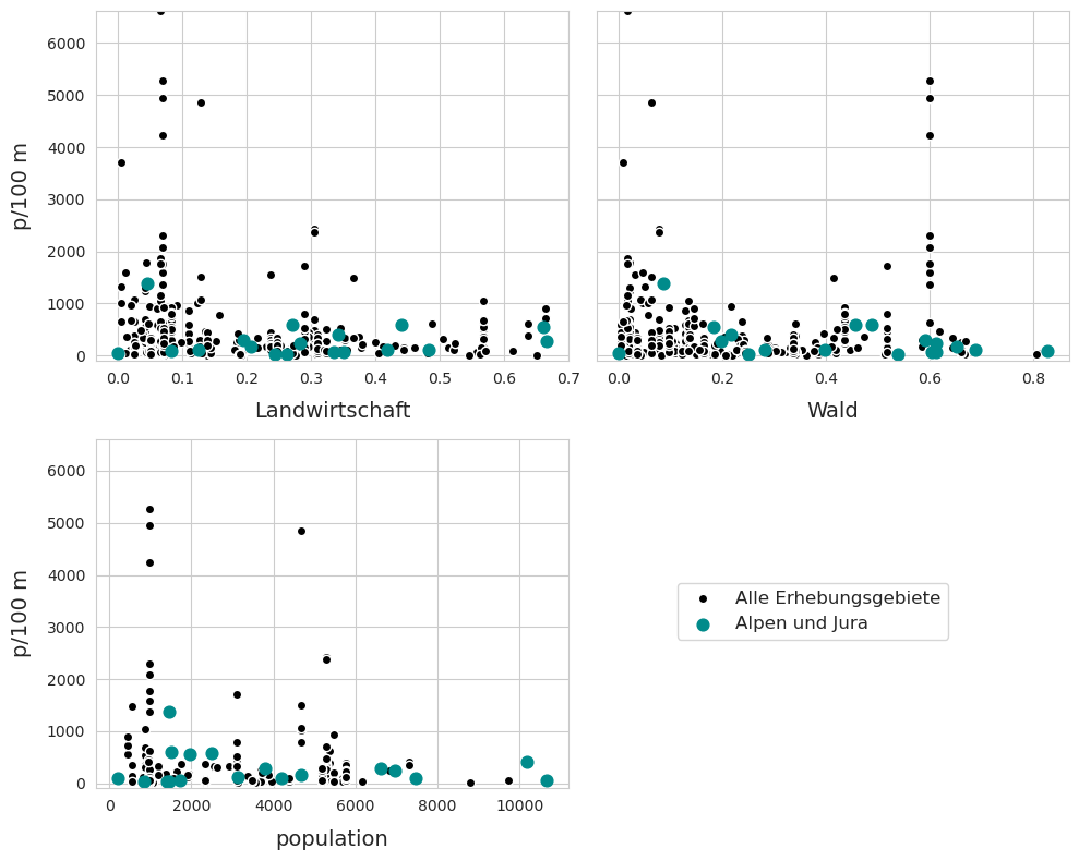
_images/f7971ff36afa7c3ea116c767156e5fc33a6750d563befce1d2037ffba4727a69.png

Abb. 2.15 #

Abbildung 2.15: Oben links: Gesamtsumme der Erhebung in Bezug auf den prozentualen Anteil an landwirtschaftlich genutzter Fläche, Bereich = (0 %, 66 %). Oben rechts: Gesamtzahl der Erhebungen in Bezug auf den Waldanteil, Bereich=(0 %, 65 %). Unten links: Gesamtzahl der Erhebungen in Bezug auf die Bevölkerung, Bereich=(199, 10668).

2.7.4. Organisation und Durchführung#

Summit foundation: Téo Gürsoy

Hammerdirt: Bettina Siegenthaler

2.7.5. Die Erhebungsorte#

	latitude	longitude	stat
standort
cabanes-des-diablerets	46.338604	7.215525	Ormont-Dessus
val-calanca	46.330718	9.120103	Calanca
san-bernardino	46.445947	9.191344	Mesocco
airolo	46.514257	8.607884	Airolo
nendaz	46.162099	7.283486	Nendaz
veysonnaz	46.180334	7.366005	Nendaz
andermatt	46.618327	8.598803	Andermatt
verbier	46.103981	7.224760	Val de Bagnes
crans-montana	46.334214	7.479386	Lens
villars	46.321937	7.073841	Ollon
les-crosets	46.183591	6.832916	Val-d'Illiez
morgins	46.236681	6.858132	Troistorrents
la-berra	46.677399	7.178738	La Roche
grindelwald	46.658523	8.065323	Grindelwald
la-tzoumaz	46.144287	7.232897	Riddes
la-robella	46.875905	6.548577	Val-de-Travers
les-diablerets	46.346141	7.151228	Ormont-Dessus
charmey	46.622641	7.189341	Val-de-Charmey
monte-generoso	45.929625	9.019921	Rovio
les-paccots	46.512592	6.949421	Châtel-Saint-Denis

2.7.6. Inventar der Objekte#

	Objekte	Objekte (St.)	Anteil	p/100 m	Häufigkeitsrate	Material
code
G704	Seilbahnbürsten	5 181	66	0	10	Plastik
G27	Zigarettenfilter	317	4	14	95	Plastik
Gfrags	Fragmentierte Kunststoffe	294	3	12	100	Plastik
G30	Snack-Verpackungen	253	3	11	95	Plastik
G705	Schrauben und Bolzen	206	2	3	65	Metall
G936	Folien für Gewächshäuser	132	1	0	15	Plastik
Gfoam	Expandiertes Polystyrol	121	1	0	20	Plastik
G93	Kabelbinder	104	1	2	60	Plastik
G200	Getränkeflaschen aus Glas, Glasfragmente	84	1	0	45	Glas
G177	Verpackungen aus Aluminiumfolie	68	0	1	60	Metall
G124	Andere Kunststoff	60	0	0	5	Plastik
G941	Verpackungsfolien, nicht für Lebensmittel	57	0	0	30	Plastik
G87	Abdeckklebeband/Verpackungsklebeband	53	0	2	60	Plastik
G204	Baumaterial; Ziegel, Rohre, Zement	49	0	0	40	Glas
G117	Styropor < 5mm	37	0	0	5	Plastik
G33	Einwegartikel; Tassen/Becher & Deckel	36	0	0	40	Plastik
G12	Kosmetika, Behälter für Körperpflegeprodukte, ...	34	0	0	5	Plastik
G89	Kunststoff-Bauabfälle	34	0	0	15	Plastik
G142	Seil, Schnur oder Netze	33	0	0	40	Stoff
G122	Kunststofffragmente (>1mm)	32	0	0	30	Plastik
G919	Nägel, Schrauben, Bolzen usw.	31	0	0	20	Metall
G922	Etiketten, Strichcodes	27	0	0	40	Plastik
G923	Taschentücher, Toilettenpapier, Servietten, Pa...	26	0	0	40	Papier
G703	Pistenmarkierungspfosten (Plastik)	21	0	0	10	Plastik
G24	Ringe von Plastikflaschen/Behältern	20	0	0	35	Plastik
G178	Kronkorken, Lasche von Dose/Ausfreisslachen	18	0	0	40	Metall
G146	Papier, Karton	18	0	0	25	Papier
G926	Kaugummi, enthält oft Kunststoffe	17	0	0	25	Plastik
G934	Sandsäcke, Kunststoff für Hochwasser- und Eros...	17	0	0	15	Plastik
G10	Lebensmittelbehälter zum einmaligen Gebrauch a...	17	0	0	15	Plastik
G34	Besteck, Teller und Tabletts	16	0	0	20	Plastik
G25	Tabak; Kunststoffverpackungen, Behälter	16	0	0	25	Plastik
G905	Haarspangen, Haargummis, persönliche Accessoir...	16	0	0	40	Plastik
G710	Ski / Snowboards (Ski, Befestigungen und ander...	15	0	0	30	Plastik
G707	Skiausrüstungsetikett	13	0	0	25	Plastik
G208	Glas oder Keramikfragmente >2.5 cm	13	0	0	25	Glas
G901	Medizinische Masken, synthetische	13	0	0	20	Plastik
G198	Andere Metallteile < 50 cm	12	0	0	40	Metall
G170	Holz (verarbeitet)	11	0	0	10	Holz
G145	Andere Textilien	11	0	0	20	Stoff
G152	Papier &Karton;Zigarettenschachteln, Papier/Ka...	11	0	0	25	Papier
G7	Getränkeflaschen < = 0,5 l	11	0	0	40	Plastik
G709	Teller von Skistock (runder Teil aus Plastik u...	11	0	0	30	Plastik
G66	Umreifungsbänder; Hartplastik für Verpackung f...	10	0	0	10	Plastik
G48	Seile, synthetische	10	0	0	20	Plastik
G100	Medizin; Behälter/Röhrchen/Verpackungen	9	0	0	40	Plastik
G31	Schleckstengel, Stengel von Lutscher	9	0	0	25	Plastik
G702	Pistenmarkierungspfosten (Holz)	9	0	0	20	Holz
G74	Schaumstoffverpackungen/Isolierung	8	0	0	10	Plastik
G129	Schläuche und Gummiplatten	8	0	0	5	Gummi
G921	Keramikfliesen und Bruchstücke	7	0	0	10	Glas
G105	Kunststofffragmente subangulär <5mm	6	0	0	5	Plastik
G23	unidentifizierte Deckel	6	0	0	10	Plastik
G20	Laschen und Deckel	6	0	0	20	Plastik
G156	Papierfragmente	6	0	0	25	Papier
G123	Polyurethan-Granulat < 5mm	6	0	0	5	Plastik
G918	Sicherheitsnadeln, Büroklammern, kleine Gebrau...	6	0	0	15	Metall
G706	Skiabonnement	5	0	0	25	Plastik
G149	Papierverpackungen	5	0	0	10	Papier
G191	Draht und Gitter	5	0	0	20	Metall
G943	Zäune Landwirtschaft, Kunststoff	4	0	0	10	Plastik
G915	Reflektoren, Mobilitätsartikel aus Kunststoff	4	0	0	5	Plastik
G175	Getränkedosen (Dosen, Getränke)	4	0	0	15	Metall
G73	Gegenstände aus Schaumstoff & Teilstücke (nich...	4	0	0	5	Plastik
G211	Sonstiges medizinisches Material	4	0	0	15	Plastik
G35	Strohhalme und Rührstäbchen	3	0	0	15	Plastik
G158	Sonstige Gegenstände aus Papier	3	0	0	15	Papier
G95	Wattestäbchen/Tupfer	3	0	0	5	Plastik
G171	Sonstiges Holz < 50cm	3	0	0	15	Holz
G194	Kabel, Metalldraht oft in Gummi- oder Kunststo...	3	0	0	10	Metall
G712	Skihandschuhe	3	0	0	10	Stoff
G711	Handwärmer	3	0	0	10	Plastik
G139	Rucksäcke	3	0	0	5	Stoff
G3	Einkaufstaschen, Shoppingtaschen	3	0	0	10	Plastik
G159	Kork	3	0	0	10	Holz
G210	Sonstiges Glas/Keramik Materialien	2	0	0	5	Glas
G90	Blumentöpfe aus Plastik	2	0	0	10	Plastik
G28	Stifte, Deckel, Druckbleistifte usw.	2	0	0	10	Plastik
G928	Bänder und Schleifen	2	0	0	5	Plastik
G931	(Absperr)band für Absperrungen, Polizei, Baust...	2	0	0	10	Plastik
G713	Skiförderband	2	0	0	5	Plastik
G26	Feuerzeug	2	0	0	10	Plastik
G155	Feuerwerkspapierhülsen und -fragmente	2	0	0	5	Papier
G181	Geschirr aus Metall, Tassen, Besteck usw.	2	0	0	5	Metall
G167	Streichhölzer oder Feuerwerke	2	0	0	5	Holz
G168	Holzbretter	2	0	0	5	Holz
G935	Gummi-Puffer für Geh- und Wanderstöcke und Tei...	1	0	0	5	Plastik
G71	Schuhe Sandalen	1	0	0	5	Plastik
G67	Industriefolie (Kunststoff)	1	0	0	5	Plastik
G148	Kartonkisten und Stücke	1	0	0	5	Papier
G65	Eimer	1	0	0	5	Plastik
G131	Gummibänder	1	0	0	5	Gummi
G8	Getränkeflaschen > 0,5L	1	0	0	5	Plastik
G128	Reifen und Antriebsriemen	1	0	0	5	Gummi
G916	Bleistifte und Bruchstücke	1	0	0	5	Holz
G917	Blähton	1	0	0	5	Glas
G929	Elektronik und Teile; Sensoren, Headsets usw.	1	0	0	5	Metall
G21	Getränke-Deckel, Getränkeverschluss	1	0	0	5	Plastik
G708	Skistöcke	1	0	0	5	Metall
G195	Batterien (Haushalt)	1	0	0	5	Metall
G101	Robidog Hundekot-Säcklein, andere Hundekotsäck...	1	0	0	5	Plastik
G199	Andere Metallteile > 50 cm	1	0	0	5	Metall
G96	Hygienebinden/Höscheneinlagen/Tampons und Appl...	1	0	0	5	Plastik
G902	Medizinische Masken, Stoff	0	0	0	0	Stoff
G9	Flaschen und Behälter für Reinigungsmittel und...	0	0	0	0	Plastik
G126	Bälle	0	0	0	0	Gummi
G900	Handschuhe Latex, persönliche Schutzausrüstung	0	0	0	0	Gummi
G125	Luftballons und Luftballonstäbchen	0	0	0	0	Gummi
G940	Schaumstoff EVA (flexibler Kunststoff)	0	0	0	0	Plastik
G88	Telefon inkl. Teile	0	0	0	0	Plastik
G904	Feuerwerkskörper; Raketenkappen	0	0	0	0	Plastik
G119	Folienartiger Kunststoff (>1mm)	0	0	0	0	Plastik
G906	Kaffeekapseln Aluminium	0	0	0	0	Metall
G907	Kaffeekapseln aus Kunststoff	0	0	0	0	Plastik
G908	Klebeband; elektrisch, isolierend	0	0	0	0	Plastik
G903	Behälter und Packungen für Handdesinfektionsmi...	0	0	0	0	Plastik
G84	CD oder CD-Hülle	0	0	0	0	Plastik
G13	Flaschen, Behälter, Fässer zum Transportieren ...	0	0	0	0	Plastik
G913	Schnuller	0	0	0	0	Plastik
G97	Behälter von Toilettenerfrischer	0	0	0	0	Plastik
G98	Windeln – Feuchttücher	0	0	0	0	Plastik
G99	Spritzen - Nadeln	0	0	0	0	Plastik
G999	Keine Gegenstände bei dieser Erhebung/Studie g...	0	0	0	0	Unbekannt
G132	Schwimmer (Angeln)	0	0	0	0	Gummi
G133	Kondome einschließlich Verpackungen	0	0	0	0	Gummi
G134	Sonstiges Gummi	0	0	0	0	Gummi
G135	Kleidung, Fussbekleidung, Kopfbedeckung, Hands...	0	0	0	0	Stoff
G136	Schuhe	0	0	0	0	Stoff
G137	Kleidung, Handtücher und Lappen	0	0	0	0	Stoff
G91	Bio-Filtermaterial / Trägermaterial aus Kunst...	0	0	0	0	Plastik
G914	Büroklammern, Wäscheklammern, Gebrauchsgegenst...	0	0	0	0	Plastik
G94	Tischtuch	0	0	0	0	Plastik
G118	Kleine Industrielle Kügelchen <5mm	0	0	0	0	Plastik
G939	Kunststoffblumen, Kunststoffpflanzen	0	0	0	0	Plastik
G938	Zahnstocher, Zahnseide Kunststoff	0	0	0	0	Plastik
G937	Pheromonköder für Weinberge	0	0	0	0	Plastik
G106	Kunststofffragmente eckig <5mm	0	0	0	0	Plastik
G104	Kunststofffragmente abgerundet / rundlich <5m...	0	0	0	0	Plastik
G942	Kunststoffspäne von Drehbänken, CNC-Bearbeitung	0	0	0	0	Plastik
G107	Zylindrische Pellets <5mm	0	0	0	0	Plastik
G933	Taschen, Etuis für Zubehör, Brillen, Elektroni...	0	0	0	0	Plastik
G932	Bio-Beads, Mikroplastik für die Abwasserbehand...	0	0	0	0	Plastik
G108	Scheibenförmige Pellets <5mm	0	0	0	0	Plastik
G930	Schaumstoff-Ohrstöpsel	0	0	0	0	Plastik
G103	Kunststofffragmente rund <5mm	0	0	0	0	Plastik
G109	Flache Pellets <5mm	0	0	0	0	Plastik
G944	Pelletmasse aus dem Spritzgussverfahren	0	0	0	0	Plastik
G11	Kosmetika für den Strand, z.B. Sonnencreme	0	0	0	0	Plastik
G927	Plastikschnur von Rasentrimmern, die zum Schne...	0	0	0	0	Plastik
G111	Kugelförmige Pellets < 5mm	0	0	0	0	Plastik
G925	Pakete: Trockenmittel/Feuchtigkeitsabsorber, m...	0	0	0	0	Plastik
G112	Industriepellets (Nurdles)	0	0	0	0	Plastik
G138	Schuhe und Sandalen	0	0	0	0	Stoff
G113	Fäden <5mm	0	0	0	0	Plastik
G114	Folien <5mm	0	0	0	0	Plastik
G92	Köderbehälter	0	0	0	0	Plastik
G115	Schaumstoff <5mm	0	0	0	0	Plastik
G116	Granulat <5mm	0	0	0	0	Plastik
G945	Rasierklingen	0	0	0	0	Metall
G102	Flip-Flops	0	0	0	0	Plastik
G183	Teile von Angelhaken	0	0	0	0	Metall
G144	Tampons	0	0	0	0	Stoff
G14	Flaschen für Motoröl (Motorölflaschen)	0	0	0	0	Plastik
G22	Deckel für Chemikalien, Reinigungsmittel (Ohne...	0	0	0	0	Plastik
G207	Tonkrüge zum Fangen von Kraken	0	0	0	0	Glas
G173	Sonstiges	0	0	0	0	Holz
G172	Sonstiges Holz > 50 cm	0	0	0	0	Holz
G17	Kartuschen von Kartuschen-spritzpistolen	0	0	0	0	Plastik
G213	Paraffinwachs	0	0	0	0	Chemikalien
G214	Öl/Teer	0	0	0	0	Chemikalien
G166	Farbpinsel	0	0	0	0	Holz
G140	Sack oder Beutel (Tragetasche), Jute oder Hanf	0	0	0	0	Stoff
G165	Glacestengel (Eisstiele), Zahnstocher, Essstäb...	0	0	0	0	Holz
G162	Kisten	0	0	0	0	Holz
G161	Verarbeitetes Holz	0	0	0	0	Holz
G29	Kämme, Bürsten und Sonnenbrillen	0	0	0	0	Plastik
G160	Paletten	0	0	0	0	Holz
G157	Papier	0	0	0	0	Papier
G205	Leuchtstoffröhren	0	0	0	0	Glas
G174	Aerosolspraydosen	0	0	0	0	Metall
G203	Geschirr aus Keramik oder Glas, Tassen, Teller...	0	0	0	0	Glas
G202	Glühbirnen	0	0	0	0	Glas
G201	Gläser, einschliesslich Stücke	0	0	0	0	Glas
G176	Konservendosen (Lebensmitteldosen)	0	0	0	0	Metall
G179	Einweg Grill	0	0	0	0	Metall
G2	Säcke, Taschen	0	0	0	0	Plastik
G180	Haushaltsgeräte	0	0	0	0	Metall
G197	sonstiges Metall	0	0	0	0	Metall
G196	Grosse metallische Gegenstände	0	0	0	0	Metall
G193	Teile von Autos und Autobatterien	0	0	0	0	Metall
G182	Angeln; Haken, Gewichte, Köder, Senkblei, usw.	0	0	0	0	Metall
G190	Farbtöpfe, Farbbüchsen, ( Farbeimer)	0	0	0	0	Metall
G19	Autoteile	0	0	0	0	Plastik
G188	Andere Kanister/Behälter < 4 L	0	0	0	0	Metall
G186	Industrieschrott	0	0	0	0	Metall
G32	Spielzeug und Partyartikel	0	0	0	0	Plastik
G154	Zeitungen oder Zeitschriften	0	0	0	0	Papier
G153	Papierbecher, Lebensmittelverpackungen aus Pap...	0	0	0	0	Papier
G55	Angelschnur (verwickelt)	0	0	0	0	Plastik
G141	Teppiche	0	0	0	0	Stoff
G143	Segel und Segeltuch	0	0	0	0	Stoff
G185	Behälter mittlerer Grösse	0	0	0	0	Metall
G70	Schrotflintenpatronen	0	0	0	0	Plastik
G147	Papiertragetaschen, (Papiertüten)	0	0	0	0	Papier
G68	Fiberglas-Fragmente	0	0	0	0	Plastik
G64	Kotflügel	0	0	0	0	Plastik
G63	Bojen	0	0	0	0	Plastik
G62	Schwimmer für Netze	0	0	0	0	Plastik
G61	Sonstiges Angelzubehör	0	0	0	0	Plastik
G60	Lichtstab, Knicklicht, Glow-sticks	0	0	0	0	Plastik
G6	Flaschen und Behälter aus Kunststoff, nicht fü...	0	0	0	0	Plastik
G59	Monofile Angelschnur (Angeln)	0	0	0	0	Plastik
G56	Verhedderte Netze	0	0	0	0	Plastik
G53	Netze und Teilstücke < 50cm	0	0	0	0	Plastik
G151	Tetrapack, Kartons	0	0	0	0	Papier
G52	Netze und Teilstücke	0	0	0	0	Plastik
G51	Fischernetz	0	0	0	0	Plastik
G50	Schnur < 1cm	0	0	0	0	Plastik
G5	Plastiksäcke/ Plastiktüten	0	0	0	0	Plastik
G49	Seile > 1cm	0	0	0	0	Plastik
G150	Milchkartons, Tetrapack	0	0	0	0	Papier
G43	Sicherheitsetiketten, Siegel für Fischerei ode...	0	0	0	0	Plastik
G41	Handschuhe Industriell/Professionell	0	0	0	0	Plastik
G40	Handschuhe Haushalt/Garten	0	0	0	0	Plastik
G4	Kleine Plastikbeutel; Gefrierbeutel, Zippsäckc...	0	0	0	0	Plastik
G39	Handschuhe	0	0	0	0	Plastik
G38	Abdeckungen; Kunststoffverpackungen, Folien zu...	0	0	0	0	Plastik
G37	Netzbeutel, Netztasche, Netzsäcke	0	0	0	0	Plastik
G36	Säcke aus strapazierfähigem Kunststoff für 25 ...	0	0	0	0	Plastik
G1	Sixpack-Ringe	0	0	0	0	Plastik

	Objekte	Objekte (St.)	Anteil	p/100 m	Häufigkeitsrate	Material
code
G702	Pistenmarkierungspfosten (Holz)	9	0	0	20	Holz
G100	Medizin; Behälter/Röhrchen/Verpackungen	9	0	0	40	Plastik
G31	Schleckstengel, Stengel von Lutscher	9	0	0	25	Plastik
G200	Getränkeflaschen aus Glas, Glasfragmente	84	1	0	45	Glas
G74	Schaumstoffverpackungen/Isolierung	8	0	0	10	Plastik
G129	Schläuche und Gummiplatten	8	0	0	5	Gummi
G921	Keramikfliesen und Bruchstücke	7	0	0	10	Glas
G177	Verpackungen aus Aluminiumfolie	68	0	1	60	Metall
G124	Andere Kunststoff	60	0	0	5	Plastik
G20	Laschen und Deckel	6	0	0	20	Plastik
G156	Papierfragmente	6	0	0	25	Papier
G105	Kunststofffragmente subangulär <5mm	6	0	0	5	Plastik
G918	Sicherheitsnadeln, Büroklammern, kleine Gebrau...	6	0	0	15	Metall
G123	Polyurethan-Granulat < 5mm	6	0	0	5	Plastik
G23	unidentifizierte Deckel	6	0	0	10	Plastik
G941	Verpackungsfolien, nicht für Lebensmittel	57	0	0	30	Plastik
G87	Abdeckklebeband/Verpackungsklebeband	53	0	2	60	Plastik
G704	Seilbahnbürsten	5 181	66	0	10	Plastik
G191	Draht und Gitter	5	0	0	20	Metall
G149	Papierverpackungen	5	0	0	10	Papier
G706	Skiabonnement	5	0	0	25	Plastik
G204	Baumaterial; Ziegel, Rohre, Zement	49	0	0	40	Glas
G73	Gegenstände aus Schaumstoff & Teilstücke (nich...	4	0	0	5	Plastik
G211	Sonstiges medizinisches Material	4	0	0	15	Plastik
G175	Getränkedosen (Dosen, Getränke)	4	0	0	15	Metall
G943	Zäune Landwirtschaft, Kunststoff	4	0	0	10	Plastik
G915	Reflektoren, Mobilitätsartikel aus Kunststoff	4	0	0	5	Plastik
G117	Styropor < 5mm	37	0	0	5	Plastik
G33	Einwegartikel; Tassen/Becher & Deckel	36	0	0	40	Plastik
G12	Kosmetika, Behälter für Körperpflegeprodukte, ...	34	0	0	5	Plastik
G89	Kunststoff-Bauabfälle	34	0	0	15	Plastik
G142	Seil, Schnur oder Netze	33	0	0	40	Stoff
G122	Kunststofffragmente (>1mm)	32	0	0	30	Plastik
G27	Zigarettenfilter	317	4	14	95	Plastik
G919	Nägel, Schrauben, Bolzen usw.	31	0	0	20	Metall
G194	Kabel, Metalldraht oft in Gummi- oder Kunststo...	3	0	0	10	Metall
G711	Handwärmer	3	0	0	10	Plastik
G712	Skihandschuhe	3	0	0	10	Stoff
G35	Strohhalme und Rührstäbchen	3	0	0	15	Plastik
G171	Sonstiges Holz < 50cm	3	0	0	15	Holz
G3	Einkaufstaschen, Shoppingtaschen	3	0	0	10	Plastik
G139	Rucksäcke	3	0	0	5	Stoff
G158	Sonstige Gegenstände aus Papier	3	0	0	15	Papier
G95	Wattestäbchen/Tupfer	3	0	0	5	Plastik
G159	Kork	3	0	0	10	Holz
Gfrags	Fragmentierte Kunststoffe	294	3	12	100	Plastik
G922	Etiketten, Strichcodes	27	0	0	40	Plastik
G923	Taschentücher, Toilettenpapier, Servietten, Pa...	26	0	0	40	Papier
G30	Snack-Verpackungen	253	3	11	95	Plastik
G703	Pistenmarkierungspfosten (Plastik)	21	0	0	10	Plastik
G705	Schrauben und Bolzen	206	2	3	65	Metall
G24	Ringe von Plastikflaschen/Behältern	20	0	0	35	Plastik
G210	Sonstiges Glas/Keramik Materialien	2	0	0	5	Glas
G28	Stifte, Deckel, Druckbleistifte usw.	2	0	0	10	Plastik
G167	Streichhölzer oder Feuerwerke	2	0	0	5	Holz
G713	Skiförderband	2	0	0	5	Plastik
G181	Geschirr aus Metall, Tassen, Besteck usw.	2	0	0	5	Metall
G90	Blumentöpfe aus Plastik	2	0	0	10	Plastik
G928	Bänder und Schleifen	2	0	0	5	Plastik
G168	Holzbretter	2	0	0	5	Holz
G931	(Absperr)band für Absperrungen, Polizei, Baust...	2	0	0	10	Plastik
G26	Feuerzeug	2	0	0	10	Plastik
G155	Feuerwerkspapierhülsen und -fragmente	2	0	0	5	Papier
G178	Kronkorken, Lasche von Dose/Ausfreisslachen	18	0	0	40	Metall
G146	Papier, Karton	18	0	0	25	Papier
G934	Sandsäcke, Kunststoff für Hochwasser- und Eros...	17	0	0	15	Plastik
G926	Kaugummi, enthält oft Kunststoffe	17	0	0	25	Plastik
G10	Lebensmittelbehälter zum einmaligen Gebrauch a...	17	0	0	15	Plastik
G25	Tabak; Kunststoffverpackungen, Behälter	16	0	0	25	Plastik
G905	Haarspangen, Haargummis, persönliche Accessoir...	16	0	0	40	Plastik
G34	Besteck, Teller und Tabletts	16	0	0	20	Plastik
G710	Ski / Snowboards (Ski, Befestigungen und ander...	15	0	0	30	Plastik
G936	Folien für Gewächshäuser	132	1	0	15	Plastik
G208	Glas oder Keramikfragmente >2.5 cm	13	0	0	25	Glas
G901	Medizinische Masken, synthetische	13	0	0	20	Plastik
G707	Skiausrüstungsetikett	13	0	0	25	Plastik
Gfoam	Expandiertes Polystyrol	121	1	0	20	Plastik
G198	Andere Metallteile < 50 cm	12	0	0	40	Metall
G709	Teller von Skistock (runder Teil aus Plastik u...	11	0	0	30	Plastik
G152	Papier &Karton;Zigarettenschachteln, Papier/Ka...	11	0	0	25	Papier
G145	Andere Textilien	11	0	0	20	Stoff
G7	Getränkeflaschen < = 0,5 l	11	0	0	40	Plastik
G170	Holz (verarbeitet)	11	0	0	10	Holz
G93	Kabelbinder	104	1	2	60	Plastik
G66	Umreifungsbänder; Hartplastik für Verpackung f...	10	0	0	10	Plastik
G48	Seile, synthetische	10	0	0	20	Plastik
G21	Getränke-Deckel, Getränkeverschluss	1	0	0	5	Plastik
G917	Blähton	1	0	0	5	Glas
G916	Bleistifte und Bruchstücke	1	0	0	5	Holz
G148	Kartonkisten und Stücke	1	0	0	5	Papier
G929	Elektronik und Teile; Sensoren, Headsets usw.	1	0	0	5	Metall
G199	Andere Metallteile > 50 cm	1	0	0	5	Metall
G195	Batterien (Haushalt)	1	0	0	5	Metall
G8	Getränkeflaschen > 0,5L	1	0	0	5	Plastik
G71	Schuhe Sandalen	1	0	0	5	Plastik
G131	Gummibänder	1	0	0	5	Gummi
G67	Industriefolie (Kunststoff)	1	0	0	5	Plastik
G96	Hygienebinden/Höscheneinlagen/Tampons und Appl...	1	0	0	5	Plastik
G101	Robidog Hundekot-Säcklein, andere Hundekotsäck...	1	0	0	5	Plastik
G65	Eimer	1	0	0	5	Plastik
G708	Skistöcke	1	0	0	5	Metall
G128	Reifen und Antriebsriemen	1	0	0	5	Gummi
G935	Gummi-Puffer für Geh- und Wanderstöcke und Tei...	1	0	0	5	Plastik
G126	Bälle	0	0	0	0	Gummi
G115	Schaumstoff <5mm	0	0	0	0	Plastik
G116	Granulat <5mm	0	0	0	0	Plastik
G904	Feuerwerkskörper; Raketenkappen	0	0	0	0	Plastik
G903	Behälter und Packungen für Handdesinfektionsmi...	0	0	0	0	Plastik
G902	Medizinische Masken, Stoff	0	0	0	0	Stoff
G118	Kleine Industrielle Kügelchen <5mm	0	0	0	0	Plastik
G119	Folienartiger Kunststoff (>1mm)	0	0	0	0	Plastik
G84	CD oder CD-Hülle	0	0	0	0	Plastik
G13	Flaschen, Behälter, Fässer zum Transportieren ...	0	0	0	0	Plastik
G88	Telefon inkl. Teile	0	0	0	0	Plastik
G900	Handschuhe Latex, persönliche Schutzausrüstung	0	0	0	0	Gummi
G113	Fäden <5mm	0	0	0	0	Plastik
G9	Flaschen und Behälter für Reinigungsmittel und...	0	0	0	0	Plastik
G906	Kaffeekapseln Aluminium	0	0	0	0	Metall
G125	Luftballons und Luftballonstäbchen	0	0	0	0	Gummi
G114	Folien <5mm	0	0	0	0	Plastik
G161	Verarbeitetes Holz	0	0	0	0	Holz
G92	Köderbehälter	0	0	0	0	Plastik
G907	Kaffeekapseln aus Kunststoff	0	0	0	0	Plastik
G942	Kunststoffspäne von Drehbänken, CNC-Bearbeitung	0	0	0	0	Plastik
G937	Pheromonköder für Weinberge	0	0	0	0	Plastik
G938	Zahnstocher, Zahnseide Kunststoff	0	0	0	0	Plastik
G939	Kunststoffblumen, Kunststoffpflanzen	0	0	0	0	Plastik
G94	Tischtuch	0	0	0	0	Plastik
G940	Schaumstoff EVA (flexibler Kunststoff)	0	0	0	0	Plastik
G103	Kunststofffragmente rund <5mm	0	0	0	0	Plastik
G102	Flip-Flops	0	0	0	0	Plastik
G908	Klebeband; elektrisch, isolierend	0	0	0	0	Plastik
G944	Pelletmasse aus dem Spritzgussverfahren	0	0	0	0	Plastik
G945	Rasierklingen	0	0	0	0	Metall
G97	Behälter von Toilettenerfrischer	0	0	0	0	Plastik
G98	Windeln – Feuchttücher	0	0	0	0	Plastik
G99	Spritzen - Nadeln	0	0	0	0	Plastik
G999	Keine Gegenstände bei dieser Erhebung/Studie g...	0	0	0	0	Unbekannt
G933	Taschen, Etuis für Zubehör, Brillen, Elektroni...	0	0	0	0	Plastik
G932	Bio-Beads, Mikroplastik für die Abwasserbehand...	0	0	0	0	Plastik
G104	Kunststofffragmente abgerundet / rundlich <5m...	0	0	0	0	Plastik
G930	Schaumstoff-Ohrstöpsel	0	0	0	0	Plastik
G106	Kunststofffragmente eckig <5mm	0	0	0	0	Plastik
G927	Plastikschnur von Rasentrimmern, die zum Schne...	0	0	0	0	Plastik
G925	Pakete: Trockenmittel/Feuchtigkeitsabsorber, m...	0	0	0	0	Plastik
G107	Zylindrische Pellets <5mm	0	0	0	0	Plastik
G108	Scheibenförmige Pellets <5mm	0	0	0	0	Plastik
G109	Flache Pellets <5mm	0	0	0	0	Plastik
G133	Kondome einschließlich Verpackungen	0	0	0	0	Gummi
G11	Kosmetika für den Strand, z.B. Sonnencreme	0	0	0	0	Plastik
G111	Kugelförmige Pellets < 5mm	0	0	0	0	Plastik
G112	Industriepellets (Nurdles)	0	0	0	0	Plastik
G914	Büroklammern, Wäscheklammern, Gebrauchsgegenst...	0	0	0	0	Plastik
G913	Schnuller	0	0	0	0	Plastik
G91	Bio-Filtermaterial / Trägermaterial aus Kunst...	0	0	0	0	Plastik
G132	Schwimmer (Angeln)	0	0	0	0	Gummi
G61	Sonstiges Angelzubehör	0	0	0	0	Plastik
G70	Schrotflintenpatronen	0	0	0	0	Plastik
G214	Öl/Teer	0	0	0	0	Chemikalien
G19	Autoteile	0	0	0	0	Plastik
G190	Farbtöpfe, Farbbüchsen, ( Farbeimer)	0	0	0	0	Metall
G151	Tetrapack, Kartons	0	0	0	0	Papier
G193	Teile von Autos und Autobatterien	0	0	0	0	Metall
G150	Milchkartons, Tetrapack	0	0	0	0	Papier
G196	Grosse metallische Gegenstände	0	0	0	0	Metall
G197	sonstiges Metall	0	0	0	0	Metall
G2	Säcke, Taschen	0	0	0	0	Plastik
G147	Papiertragetaschen, (Papiertüten)	0	0	0	0	Papier
G201	Gläser, einschliesslich Stücke	0	0	0	0	Glas
G202	Glühbirnen	0	0	0	0	Glas
G203	Geschirr aus Keramik oder Glas, Tassen, Teller...	0	0	0	0	Glas
G205	Leuchtstoffröhren	0	0	0	0	Glas
G207	Tonkrüge zum Fangen von Kraken	0	0	0	0	Glas
G144	Tampons	0	0	0	0	Stoff
G188	Andere Kanister/Behälter < 4 L	0	0	0	0	Metall
G186	Industrieschrott	0	0	0	0	Metall
G185	Behälter mittlerer Grösse	0	0	0	0	Metall
G173	Sonstiges	0	0	0	0	Holz
G165	Glacestengel (Eisstiele), Zahnstocher, Essstäb...	0	0	0	0	Holz
G166	Farbpinsel	0	0	0	0	Holz
G160	Paletten	0	0	0	0	Holz
G157	Papier	0	0	0	0	Papier
G17	Kartuschen von Kartuschen-spritzpistolen	0	0	0	0	Plastik
G172	Sonstiges Holz > 50 cm	0	0	0	0	Holz
G174	Aerosolspraydosen	0	0	0	0	Metall
G183	Teile von Angelhaken	0	0	0	0	Metall
G154	Zeitungen oder Zeitschriften	0	0	0	0	Papier
G176	Konservendosen (Lebensmitteldosen)	0	0	0	0	Metall
G153	Papierbecher, Lebensmittelverpackungen aus Pap...	0	0	0	0	Papier
G179	Einweg Grill	0	0	0	0	Metall
G180	Haushaltsgeräte	0	0	0	0	Metall
G182	Angeln; Haken, Gewichte, Köder, Senkblei, usw.	0	0	0	0	Metall
G213	Paraffinwachs	0	0	0	0	Chemikalien
G22	Deckel für Chemikalien, Reinigungsmittel (Ohne...	0	0	0	0	Plastik
G68	Fiberglas-Fragmente	0	0	0	0	Plastik
G143	Segel und Segeltuch	0	0	0	0	Stoff
G49	Seile > 1cm	0	0	0	0	Plastik
G5	Plastiksäcke/ Plastiktüten	0	0	0	0	Plastik
G50	Schnur < 1cm	0	0	0	0	Plastik
G51	Fischernetz	0	0	0	0	Plastik
G52	Netze und Teilstücke	0	0	0	0	Plastik
G53	Netze und Teilstücke < 50cm	0	0	0	0	Plastik
G55	Angelschnur (verwickelt)	0	0	0	0	Plastik
G56	Verhedderte Netze	0	0	0	0	Plastik
G59	Monofile Angelschnur (Angeln)	0	0	0	0	Plastik
G6	Flaschen und Behälter aus Kunststoff, nicht fü...	0	0	0	0	Plastik
G60	Lichtstab, Knicklicht, Glow-sticks	0	0	0	0	Plastik
G162	Kisten	0	0	0	0	Holz
G62	Schwimmer für Netze	0	0	0	0	Plastik
G63	Bojen	0	0	0	0	Plastik
G64	Kotflügel	0	0	0	0	Plastik
G43	Sicherheitsetiketten, Siegel für Fischerei ode...	0	0	0	0	Plastik
G41	Handschuhe Industriell/Professionell	0	0	0	0	Plastik
G40	Handschuhe Haushalt/Garten	0	0	0	0	Plastik
G136	Schuhe	0	0	0	0	Stoff
G141	Teppiche	0	0	0	0	Stoff
G140	Sack oder Beutel (Tragetasche), Jute oder Hanf	0	0	0	0	Stoff
G14	Flaschen für Motoröl (Motorölflaschen)	0	0	0	0	Plastik
G29	Kämme, Bürsten und Sonnenbrillen	0	0	0	0	Plastik
G138	Schuhe und Sandalen	0	0	0	0	Stoff
G137	Kleidung, Handtücher und Lappen	0	0	0	0	Stoff
G32	Spielzeug und Partyartikel	0	0	0	0	Plastik
G4	Kleine Plastikbeutel; Gefrierbeutel, Zippsäckc...	0	0	0	0	Plastik
G135	Kleidung, Fussbekleidung, Kopfbedeckung, Hands...	0	0	0	0	Stoff
G134	Sonstiges Gummi	0	0	0	0	Gummi
G36	Säcke aus strapazierfähigem Kunststoff für 25 ...	0	0	0	0	Plastik
G37	Netzbeutel, Netztasche, Netzsäcke	0	0	0	0	Plastik
G38	Abdeckungen; Kunststoffverpackungen, Folien zu...	0	0	0	0	Plastik
G39	Handschuhe	0	0	0	0	Plastik
G1	Sixpack-Ringe	0	0	0	0	Plastik