Show code cell source
%load_ext watermark
# sys, file and nav packages:
import datetime as dt
import json
import functools
import time

# math packages:
import pandas as pd
import numpy as np
from scipy import stats
from statsmodels.distributions.empirical_distribution import ECDF

# charting:
import matplotlib as mpl
import matplotlib.pyplot as plt
import matplotlib.dates as mdates
from matplotlib import ticker
from matplotlib import colors
from matplotlib.colors import LinearSegmentedColormap
from matplotlib.gridspec import GridSpec
from mpl_toolkits.axes_grid1 import make_axes_locatable
from mpl_toolkits.axes_grid1.inset_locator import inset_axes

import seaborn as sns

import IPython
from PIL import Image as PILImage
from IPython.display import Markdown as md
from IPython.display import display
from myst_nb import glue

import time

start_date = '2020-03-01'
end_date ='2021-05-31'

a_qty = 20

a_fail_rate = .5

use_fail = False

unit_label = 'p/100m'

# survey data:
dfx= pd.read_csv('resources/checked_sdata_eos_2020_21.csv')


dfBeaches = pd.read_csv("resources/beaches_with_land_use_rates.csv")
dfCodes = pd.read_csv("resources/codes_with_group_names_2015.csv")

# set the index of the beach data to location slug
dfBeaches.set_index('slug', inplace=True)

# set the index of to codes
dfCodes.set_index("code", inplace=True)

# code description map
code_d_map = dfCodes.description

# code material map
code_m_map = dfCodes.material

def scaleTheColumn(x):

    xmin = x.min()
    xmax = x.max()
    xscaled = (x-xmin)/(xmax-xmin)

    return xscaled


# this defines the css rules for the note-book table displays
header_row = {'selector': 'th:nth-child(1)', 'props': f'background-color: #FFF;'}
even_rows = {"selector": 'tr:nth-child(even)', 'props': f'background-color: rgba(139, 69, 19, 0.08);'}
odd_rows = {'selector': 'tr:nth-child(odd)', 'props': 'background: #FFF;'}
table_font = {'selector': 'tr', 'props': 'font-size: 12px;'}
table_css_styles = [even_rows, odd_rows, table_font, header_row]
1. All Data and all locations: original maps#
In the original report the boundary of land use effects was limited to the topographical features within a radius of 1’500 m from the survey location. The purpose of this work is to quantify how the correlation between survey results and land use changes as we consider greater distances from the survey location.
All locations with land use data are considered (see notes)
Surveys from rivers and lakes are considered as a single group
The original work is reproduced here, using the map (cartographic) features available in 2019. For this example progressively more amounts of land were considered for each survey location. The radius from the survey location is increased by 500 m from the initial 1500 m up to 5 000 m. At 5 000 meters we skip a step and do one last test at 10k.
The results at each radius are compared by number of correlations.This is for informational purposes and serves as guide to the proceeding chapters where the updated maps from 2022 are used.
1.1. Notes#
excluded data
At the time the report was published we did not have access to the land use data around Walensee. The good news is that it is now available with the most recent download. However, for this example the data from Walensee is excluded. This includes all samples that were taken in the region represented in the map below.
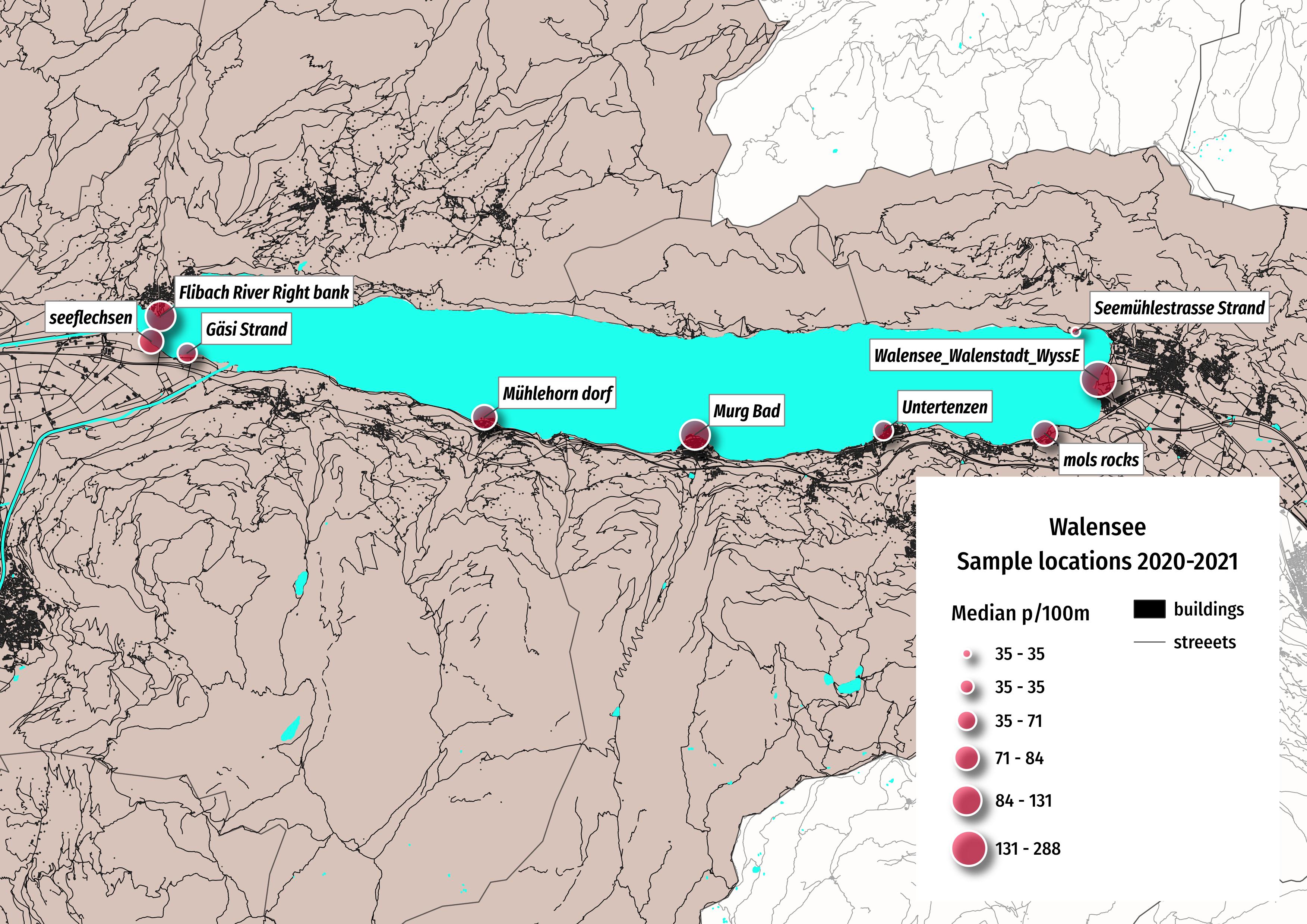
Fig. 1.1 #
figure 1.1: Detail of the survey area for where there was no land use data.
objects of interest
The objects of interest are defined as those objects where 20 or more were collected at one or more surveys. In reference to the default data: that is the value of the quantity column:
Show code cell source
pdtype = pd.core.frame.DataFrame
pstype = pd.core.series.Series


new_label_keys = {
    1:"industrial",
    2:"buildings",
    3:"buildings",
    4:"buildings",
    5:"buildings",
    6:"transport",
    7:"transport",
    8:"transport",
    9:"buildings",
    10:"recreation",
    11:"agriculture",
    12:"agriculture",
    13:"agriculture",
    14:"agriculture",
    15:"agriculture",
    16:"agriculture",
    17:"woods",
    18:"agriculture",
    19:"woods",
    20:"woods",
    21:"woods",
    22:"woods",
    23:"water",
    24:"water",
    25:"unproductive",
    26:"unproductive",
    27:"unproductive"
}


def combineLandUseFeatures(buffer_data: pdtype = None, a_col: str = "AS18_27", new_col: str = "label",
                           new_label_keys: dict = new_label_keys) -> pdtype:
    """Assigns labels to landuse values according to <label_keys_new>. The new labels,
    when aggregated, create groups of landuse values that are similar. For exmaple,
    all the different types of buildings are labeled "buildings"

    Args:
        buffer_data: The land use values at a given radius
        a_col: The original column name that holds the labels for the land use values
        new_col: The new name of the column with the new labels

    Returns:
        The data frame with the new column and the new labels
    """

    buffer_data.rename(columns={"slug":"location", a_col:new_col}, inplace=True)
    buffer_data[new_col] = buffer_data[new_col].apply(lambda x : new_label_keys[x])

    return buffer_data

def adjustLandUse(buffer_data: pdtype = None, exclude_these: list = [], locations: list = []) -> pdtype:
    """The surface area of the water feature is removed from landuse calcluation. This
    can be bypassed. However, the study considers the surface area of the water as a fixed
    feature that exchanges with the different landuse features (which are not fixed).

    Args:
        buffer_data: The land use values at a given radius
        exclude_these: The labels to be excluded from the land use total
        locations: The locations of interest with buffer data

    Returns:
        The dataframe with the locations in locations and without the excluded labels
    """
    data = buffer_data[~buffer_data.label.isin(exclude_these)]
    data = data[data.location.isin(locations)]

    return data

def addRoadLengthToBuffer(buffer_data: pdtype = None, location: str = None,
                          road_lengths: pstype = None, scale: float = 1000.0):
    """Adds the length of road network to the % land use values.
    """

    road_length = road_lengths.loc[location]
    if scale != 1:
        road_length = round(road_length/scale, 1)

    buffer_data["roads"] = road_length

    return buffer_data

def addIntersectsToBuffer(buffer_data: pdtype = None, location: str = None,
                          intersects: pstype = None, scale: float = 100.0):

    """Adds the number of river intersections to the buffer.

    The river intersections are the points where rivers join the body of water of interest
    """

    n_intersects = intersects.loc[location]

    buffer_data["intersects"] = n_intersects

    return buffer_data


def calculatePercentLandUse(buffer_data: pdtype = None, location: str = None, label: str = "label",
                           add_intersects_roads: bool = True,  road_lengths: pstype = None, intersects: pstype = None,) -> pd.Series:
    """Figures the % of total of each landuse feature for one location.

    Args:
        buffer_data: The land use values at a given radius
        location: The survey location of interest

    Returns:
        A pandas series of the % of total for each landuse feature in the index
    """

    try:
        # try to reitrieve the land use data for a location
        location_data = buffer_data[buffer_data.location == location][label].value_counts()
    except ValueError:
        print("The location data could not retrieved")
        raise

    # the sum of all land use features in the radius
    total = location_data.sum()
    # the amount of the area attributed to water (lakes and rivers)
    water = location_data.loc["water"]
    # divide the land_use values by the total minus the amount attributed to water
    results = location_data/(total-water)
    # name the series
    results.name = location
    # the intersects and road-lengths are calculated seprately
    # if add_intersects and roads is true, attach them to the
    # the land use values
    if add_intersects_roads:
        results = addIntersectsToBuffer(buffer_data=results, location=location, intersects=intersects)
        results = addRoadLengthToBuffer(buffer_data=results, location=location, road_lengths=road_lengths)


    return results

class BufferData:
    a_col="AS18_27"
    new_col = "label"
    exclude_these = []
    label_keys = new_label_keys
    beach_data = dfBeaches


    def __init__(self, file_name: str = None, locations: list = []):
        self.buffer = pd.read_csv(file_name)
        self.buffer_data = combineLandUseFeatures(buffer_data=self.buffer, a_col=self.a_col, new_col=self.new_col)
        self.adjusted_buffer = adjustLandUse(buffer_data=self.buffer_data, exclude_these=self.exclude_these, locations=locations)
        self.pctLandUse = None
        self.locations = locations

    def percentLandUse(self):

        if isinstance(self.pctLandUse, pdtype):
            return self.pctLandUse

        if isinstance(self.adjusted_buffer, pdtype):
            results = []
            road_lengths = self.beach_data.streets
            intersects = self.beach_data.intersects
            for location in self.locations:
                result = calculatePercentLandUse(buffer_data=self.adjusted_buffer, location=location, road_lengths=road_lengths, intersects=intersects)
                results.append(result)
        else:
            raise TypeError

        self.pctLandUse = pd.concat(results, axis=1)

        return self.pctLandUse

def timer(func):
    @functools.wraps(func)
    def wrapper(*args, **kwargs):
        start_time = time.perf_counter()
        value = func(*args, **kwargs)
        end_time = time.perf_counter()
        run_time = end_time - start_time
        print("Finished {} in {} secs".format(repr(func.__name__), round(run_time, 3)))
        return value

    return wrapper

def assignLanduseValue(sample: pstype=None, land_use: str=None) -> float:
    # returns the requested value of land use from the sample
    # if the requested landuse value is not present in the buffer
    # zero is returned
    try:
        result = sample.loc[land_use]
    except KeyError:
        result = 0

    return result

def cleanSurveyResults(data):
    # performs data cleaning operations on the
    # default data

    data['loc_date'] = list(zip(data.location, data["date"]))
    data['date'] = pd.to_datetime(data["date"])

    # get rid of microplastics
    mcr = data[data.groupname == "micro plastics (< 5mm)"].code.unique()

    # replace the bad code
    data.code = data.code.replace('G207', 'G208')
    data = data[~data.code.isin(mcr)]

    # walensee has no landuse values
    data = data[data.water_name_slug != 'walensee']

    return data

class SurveyResults:
    """Creates a dataframe from a valid filename. Assigns the column names and defines a list of
    codes and locations that can be used in the CodeData class.
    """

    file_name = 'resources/checked_sdata_eos_2020_21.csv'
    columns_to_keep=[
        'loc_date',
        'location',
        'river_bassin',
        'water_name_slug',
        'city',
        'w_t',
        'intersects',
        'code',
        'pcs_m',
        'quantity'
    ]

    def __init__(self, data: str = file_name, clean_data: bool = True, columns: list = columns_to_keep, w_t: str = None):
        self.dfx = pd.read_csv(data)
        self.df_results = None
        self.locations = None
        self.valid_codes = None
        self.clean_data = clean_data
        self.columns = columns
        self.w_t = w_t

    def validCodes(self):
        # creates a list of unique code values for the data set
        conditions = [
            isinstance(self.df_results, pdtype),
            "code" in self.df_results.columns
        ]

        if all(conditions):

            try:
                valid_codes = self.df_results.code.unique()
            except ValueError:
                print("There was an error retrieving the unique code names, self.df.code.unique() failed.")
                raise
            else:
                self.valid_codes = valid_codes


    def surveyResults(self):

        # if this method has been called already
        # return the result
        if self.df_results is not None:
            return self.df_results

        # for the default data self.clean data must be called
        if self.clean_data is True:
            fd = cleanSurveyResults(self.dfx)

        # if the data is clean then if can be used directly
        else:
            fd = self.dfx

        # filter the data by the variable w_t
        if self.w_t is not None:
            fd = fd[fd.w_t == self.w_t]

        # keep only the required columns
        if self.columns:
            fd = fd[self.columns]

        # assign the survey results to the class attribute
        self.df_results = fd

        # define the list of codes in this df
        self.validCodes()

        return self.df_results

    def surveyLocations(self):
        if self.locations is not None:
            return self.locations
        if self.df_results is not None:
            self.locations = self.dfResults.location.unique()
            return self.locations
        else:
            print("There is no survey data loaded")
            return None


class CodeData:

    def __init__(self, data: pdtype = None, code: str = None, **kwargs):

        self.data = data
        self.code = code
        self.code_data = None

    def makeCodeData(self)->pdtype:

        if isinstance(self.code_data, pdtype):
            return self.code_data

        conditions = [
            isinstance(self.data, pdtype)
        ]

        if all(conditions):
            self.code_data = self.data[self.data.code == self.code]
            return self.code_data

class CodeResults:

    def __init__(self, code_data: pdtype = None, buffer: pdtype = None, code: str = None,
                 method: callable = stats.spearmanr, **kwargs):

        self.code_data = code_data
        self.buffer = buffer
        self.code = code
        self.method = method
        self.y = None
        self.x = None
        super().__init__()


    def landuseValueForOneCondition(self, land_use: str = None, locations: list = None)-> (np.array, np.array):

        x = self.code_data.pcs_m.values
        y = [self.buffer[x].loc[land_use] for x in self.code_data.location.values]
        self.x, self.y = x, np.array(y)

        return self.x, self.y

    def rhoForALAndUseCategory(self, x: np.ndarray = None, y: np.ndarray = None) -> (float, float):
        # returns the asymptotic results if ranking based method is used
        c, p = self.method(x, y)
        return c, p

    def getRho(self, x: np.array = None)-> float:
        # assigns y from self
        result = self.method(x, self.y)

        return result.correlation

    def exactPValueForRho(self)-> float:
        # perform a permutation test instead of relying on
        # the asymptotic p-value. Only one of the two inputs
        # needs to be shuffled.
        p = stats.permutation_test((self.x,) , self.getRho, permutation_type='pairings', n_resamples=1000)

        return p


def makeBufferObject(file_name: str = "resources/buffer_output/luse_1500.csv", buffer_locations: list = None) -> (pdtype, pdtype):
    # Makes a buffer object by calling the BufferData class
    # calls the percentLandUse method and fills Nan values
    # returns the buffer_data object and pct land use values

    buffer_data = BufferData(file_name=file_name, locations=buffer_locations)
    pct_vals = buffer_data.percentLandUse()
    pct_vals.fillna(0, inplace=True)

    return buffer_data, pct_vals

def asymptoticAndExactPvalues(data: pdtype = None, buffer: pdtype = None, code: 'str'=None, land_use: 'str'=None)-> dict:

    code_data = CodeData(data=data, code=code).makeCodeData()
    code_results = CodeResults(code_data=code_data, buffer=buffer)

    x, y = code_results.landuseValueForOneCondition(land_use=land_use)
    ci, pi = code_results.rhoForALAndUseCategory(x, y)
    px = code_results.exactPValueForRho()

    return {"code": code, "landuse": land_use, "a_symp": (round(pi, 3), ci), "exact": (round(px.pvalue, 3), px.statistic,)}

@timer
def rhoForOneBuffer(data: pdtype = None, buffer_file: str = "resources/buffer_output/luse_1500.csv",
                    codes: list=None, land_use: list=None)->(list, pdtype, pdtype):

    buffer_locations = data.location.unique()
    new_buffer, buffer_vals = makeBufferObject(file_name=buffer_file, buffer_locations=buffer_locations)

    rhovals_for_this_buffer = []
    for code in codes:
        for use in land_use:
            results = asymptoticAndExactPvalues(data=data, buffer=buffer_vals, code=code, land_use=use)
            rhovals_for_this_buffer.append(results)

    return rhovals_for_this_buffer, new_buffer, buffer_vals

def resultsDf(rhovals: pdtype = None, pvals: pdtype = None)-> pdtype:
    results_df = []
    for i, n in enumerate(pvals.index):
        arow_of_ps = pvals.iloc[i]
        p_fail = arow_of_ps[ arow_of_ps > 0.05]
        arow_of_rhos = rhovals.iloc[i]

        for label in p_fail.index:
            arow_of_rhos[label] = 0
        results_df.append(arow_of_rhos)

    return results_df

def rotateText(x):
    return 'writing-mode: vertical-lr; transform: rotate(-180deg);  padding:10px; margins:0; vertical-align: baseline;'

def nObjectsPerLandUse(uses,surveys):
    results = {}
    for a_use in uses.index:
        total = surveys[surveys.code.isin(uses.loc[a_use])].quantity.sum()
        results.update({a_use:total})

    return pd.DataFrame(index=results.keys(), data=results.values(), columns=["total"])

fdx = SurveyResults()
df = fdx.surveyResults()

location_no_luse = ["linth_route9brucke",
                "seez_spennwiesenbrucke",
                'limmat_dietikon_keiserp',
                "seez"]

city_no_luse = ["Walenstadt", "Weesen", "Glarus Nord", "Quarten"]

df = df[~df.location.isin(location_no_luse)]
df = df[~df.city.isin(city_no_luse)]

df[["location","city", "water_name_slug","loc_date", "code", "pcs_m", "quantity"]].head().style.set_table_styles(table_css_styles)
| location | city | water_name_slug | loc_date | code | pcs_m | quantity | |
|---|---|---|---|---|---|---|---|
| 0 | maladaire | La Tour-de-Peilz | lac-leman | ('maladaire', '2021-05-01') | G191 | 0.010000 | 1 |
| 1 | maladaire | La Tour-de-Peilz | lac-leman | ('maladaire', '2021-05-01') | G35 | 0.010000 | 1 |
| 2 | maladaire | La Tour-de-Peilz | lac-leman | ('maladaire', '2021-05-01') | G21 | 0.010000 | 1 |
| 3 | maladaire | La Tour-de-Peilz | lac-leman | ('maladaire', '2021-05-01') | G67 | 0.030000 | 2 |
| 4 | maladaire | La Tour-de-Peilz | lac-leman | ('maladaire', '2021-05-01') | G23 | 0.010000 | 1 |
In the report the objects of interest were either in the top ten by quantity and/or found in at least 50% of the samples. Consider the research question when filtering the objects. A filter can be based on use as well as abundance or frequency.
percent attributed to buildings
Originally the % of land attributed to buildings was calculated by summing the area of each topographical representation of a building from the map layer. In this example the % attributed to buildings is calculated the same as forests, agriculture, unproductive, recreation and industrial. The number of 100 m squares attributed to citys was divided by the total number of 100 m squares in the buffer (minus the number of squares attributed to water).
1.2. The survey data#
The sampling period for the IQAASL project started in April 2020 and ended May 2021.
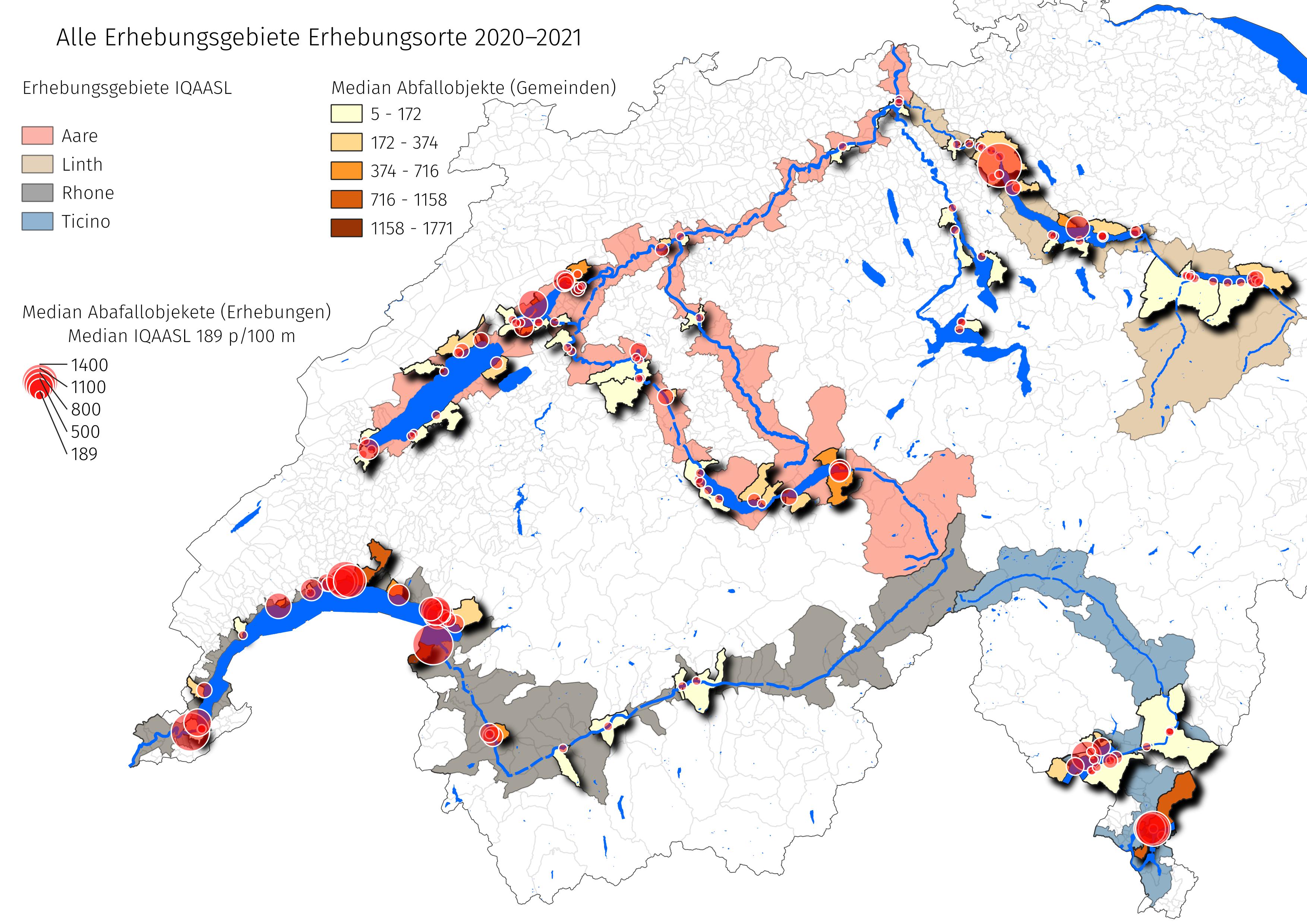
Fig. 1.2 #
figure 1.2: All survey locations IQAASL.
Summary data of the surveys, not including locations in the Walensee area:
Show code cell source
## The survey results
locations = df.location.unique()
samples = df.loc_date.unique()
lakes = df[df.w_t == "l"].drop_duplicates("loc_date").w_t.value_counts().values[0]
river = df[df.w_t == "r"].drop_duplicates("loc_date").w_t.value_counts().values[0]
codes_identified = df[df.quantity > 0].code.unique()
codes_possible = df.code.unique()
total_id = df.quantity.sum()

data_summary = {
    "n locations": len(locations),
    "n samples": len(samples),
    "n lake samples": lakes,
    "n river samples": river,
    "n identified object types": len(codes_identified),
    "n possible object types": len(codes_possible),
    "total number of objects": total_id
}

pd.DataFrame(index = data_summary.keys(), data=data_summary.values()).style.set_table_styles(table_css_styles)
| 0 | |
|---|---|
| n locations | 128 |
| n samples | 349 |
| n lake samples | 300 |
| n river samples | 49 |
| n identified object types | 191 |
| n possible object types | 211 |
| total number of objects | 46832 |
1.3. Land use correlation#
1.3.1. Example: object = cigarette ends, landuse = buildings v/s agg#
When the survey results for cigarette ends are considered with respect to the percent of land attributed to buildings or agriculture the it appears that cigartette ends accumulate at different rates depending on the landuse. The plot below. demonstrates the relationship of the survey values under the two conditions.
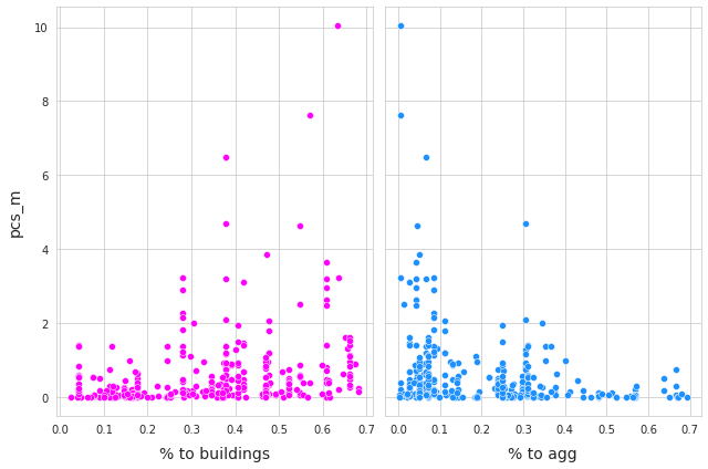
Fig. 1.3 #
figure 1.3: Left: survey totals cigarette ends with respect to % of land to buildings. = 0.39, p-value < .001. Right: survey totals cigarette ends with respect to % of land to aggriculture. = -0.31, p-value < .001.
This relationship is considered for all the objects of interest. As the value of rho increases the points tend to accumulate to the right of the chart, it is the opposite as rho approaches -1.
1.3.2. Land use correlation @ 1500 m#
Show code cell source
no_luse_data = ["linth_route9brucke",
                "seez_spennwiesenbrucke",
                'limmat_dietikon_keiserp',
                "seez"]

df = df[~df.location.isin(no_luse_data)]

# the land use features we are interested in
land_use =["buildings",  "industrial", "roads", "recreation", "agriculture","woods", "intersects", "unproductive"]

# codes of interest
# we are interested in objects that were found in 1/2 surveys
fail = .5

# calculate the frequency that each code was found
codes_fail = df[df.quantity > 20].code.unique()

# identify the land_use data
buffer_file = "resources/buffer_output/luse_1500.csv"

# make the buffer and get the coeficients
rho_vals, new_buffer, buffer_vals = rhoForOneBuffer(data=df, buffer_file=buffer_file , codes=codes_fail, land_use=land_use)
Finished 'rhoForOneBuffer' in 118.484 secs
Show code cell source
buffer_results = [{"code":x["code"], "use": x["landuse"], "exact_p": x["exact"][0], "p": x["a_symp"][0], "rho": x["exact"][1]} for x in rho_vals]
rho_at_buffer = pd.DataFrame(buffer_results)

pvals = rho_at_buffer.pivot_table(index="code", columns="use", values="exact_p", aggfunc='first')
rhovals = rho_at_buffer.pivot_table(index="code", columns="use", values="rho", aggfunc='first').round(3)

buffer_results = pd.DataFrame(resultsDf(rhovals, pvals))
buffer_results.columns.name = None
bfr = buffer_results.style.format(precision=2).set_table_styles(table_css_styles)
bfr = bfr.background_gradient(axis=None, vmin=buffer_results.min().min(), vmax=buffer_results.max().max(), cmap="coolwarm")
bfr = bfr.applymap_index(rotateText, axis=1)

glue("rho_at_1500", bfr, display=False)
| agriculture | buildings | industrial | intersects | recreation | roads | unproductive | woods | |
|---|---|---|---|---|---|---|---|---|
| G10 | -0.16 | 0.00 | 0.00 | 0.13 | 0.00 | 0.00 | -0.11 | 0.00 |
| G137 | 0.00 | 0.00 | -0.12 | 0.00 | 0.00 | 0.00 | 0.00 | 0.00 |
| G149 | -0.11 | 0.00 | 0.00 | 0.00 | 0.00 | 0.00 | -0.13 | 0.00 |
| G155 | 0.00 | 0.00 | 0.00 | 0.00 | 0.00 | 0.00 | 0.00 | 0.00 |
| G177 | -0.34 | 0.27 | 0.11 | 0.00 | 0.34 | 0.33 | -0.23 | -0.15 |
| G178 | -0.42 | 0.41 | 0.00 | -0.21 | 0.24 | 0.27 | -0.39 | -0.17 |
| G200 | -0.23 | 0.21 | -0.14 | 0.00 | 0.00 | 0.00 | -0.13 | 0.00 |
| G204 | 0.00 | 0.00 | 0.00 | 0.00 | 0.00 | 0.00 | 0.00 | 0.00 |
| G208 | -0.10 | 0.10 | 0.00 | 0.00 | 0.00 | 0.00 | -0.09 | -0.09 |
| G21 | -0.13 | 0.00 | 0.00 | 0.11 | 0.13 | 0.00 | 0.00 | 0.00 |
| G22 | 0.00 | 0.00 | 0.00 | 0.00 | 0.00 | 0.00 | 0.00 | 0.00 |
| G23 | 0.00 | 0.00 | 0.00 | 0.12 | 0.12 | 0.00 | 0.00 | 0.00 |
| G24 | -0.12 | 0.13 | 0.00 | 0.00 | 0.13 | 0.00 | -0.19 | -0.13 |
| G25 | -0.13 | 0.12 | 0.00 | 0.11 | 0.12 | 0.00 | 0.00 | -0.12 |
| G27 | -0.33 | 0.37 | 0.10 | 0.00 | 0.33 | 0.19 | -0.34 | -0.22 |
| G3 | -0.12 | 0.00 | 0.14 | 0.00 | 0.00 | 0.00 | 0.00 | 0.12 |
| G30 | -0.26 | 0.22 | 0.11 | 0.00 | 0.27 | 0.00 | -0.17 | -0.22 |
| G38 | 0.00 | 0.00 | 0.00 | 0.00 | 0.00 | 0.00 | 0.00 | 0.00 |
| G67 | 0.00 | 0.00 | 0.00 | 0.24 | 0.00 | -0.11 | 0.00 | 0.00 |
| G70 | -0.12 | 0.00 | 0.00 | 0.14 | 0.00 | 0.00 | -0.12 | 0.00 |
| G73 | -0.10 | 0.00 | 0.00 | 0.00 | 0.00 | 0.00 | 0.00 | 0.00 |
| G74 | -0.16 | 0.00 | 0.00 | 0.13 | 0.19 | 0.00 | -0.17 | 0.00 |
| G89 | -0.13 | 0.00 | 0.00 | 0.14 | 0.00 | 0.00 | 0.00 | 0.00 |
| G904 | 0.11 | -0.16 | -0.14 | 0.19 | 0.00 | -0.17 | 0.18 | 0.21 |
| G921 | -0.12 | 0.00 | 0.00 | 0.00 | -0.15 | 0.00 | -0.23 | 0.00 |
| G922 | 0.00 | 0.00 | 0.00 | 0.00 | 0.18 | 0.00 | 0.00 | 0.00 |
| G923 | -0.17 | 0.16 | 0.00 | 0.00 | 0.12 | 0.15 | -0.14 | 0.00 |
| G928 | 0.00 | 0.00 | 0.00 | 0.00 | 0.00 | 0.00 | 0.00 | 0.00 |
| G940 | 0.00 | 0.00 | 0.00 | 0.00 | 0.00 | 0.00 | 0.00 | 0.10 |
| G941 | 0.00 | 0.00 | 0.00 | 0.11 | 0.14 | 0.00 | 0.17 | 0.00 |
| G944 | 0.00 | -0.14 | 0.00 | 0.14 | 0.00 | 0.00 | 0.00 | 0.00 |
| G95 | -0.15 | 0.00 | 0.00 | 0.00 | 0.18 | 0.00 | -0.21 | 0.00 |
| G96 | 0.00 | 0.00 | 0.00 | 0.00 | 0.00 | 0.00 | 0.00 | 0.00 |
| G98 | -0.16 | 0.00 | 0.15 | -0.24 | 0.18 | 0.20 | -0.12 | 0.00 |
| Gfoam | 0.00 | 0.00 | 0.00 | 0.25 | 0.00 | -0.19 | 0.00 | 0.00 |
| Gfrags | 0.00 | 0.00 | 0.00 | 0.21 | 0.18 | 0.00 | 0.00 | 0.00 |
Fig. 1.4 #
Figure 1.4: The corelation coeficient of trash density to landuse features for All data. Coeffecients of 0 indicate that there is no statistical indication that the land use feature has an effect (positive or negative) on the trash density.
Show code cell source
def collectBufferResultsRhoAndPvals(rho_vals):
    buffer_results = [{"code":x["code"], "use": x["landuse"], "exact_p": x["exact"][0], "p": x["a_symp"][0], "rho": x["exact"][1]} for x in rho_vals]
    rho_at_buffer = pd.DataFrame(buffer_results)

    pvals = rho_at_buffer.pivot_table(index="code", columns="use", values="exact_p", aggfunc='first')
    rhovals = rho_at_buffer.pivot_table(index="code", columns="use", values="rho", aggfunc='first').round(3)
    buffer_results = pd.DataFrame(resultsDf(rhovals, pvals))

    return rho_at_buffer, pvals, rhovals, buffer_results

def styleBufferResults(buffer_results):
    buffer_results.columns.name = None
    bfr = buffer_results.style.format(precision=2).set_table_styles(table_css_styles)
    bfr = bfr.background_gradient(axis=None, vmin=buffer_results.min().min(), vmax=buffer_results.max().max(), cmap="coolwarm")
    bfr = bfr.applymap_index(rotateText, axis=1)

    return bfr
1.3.3. Land use correlation @ 2 000 m#
Show code cell source
# identify the land_use data
buffer_file = "resources/buffer_output/luse_2000.csv"

# make the buffer and get the coeficients
rho_vals_2k, new_buffer_2k, buffer_vals_2k = rhoForOneBuffer(data=df, buffer_file=buffer_file , codes=codes_fail, land_use=land_use)

rho_at_2k, pvals2k, rhovals2k, buffer_results2k = collectBufferResultsRhoAndPvals(rho_vals_2k)
styleBufferResults(buffer_results2k)
Finished 'rhoForOneBuffer' in 124.526 secs
| agriculture | buildings | industrial | intersects | recreation | roads | unproductive | woods | |
|---|---|---|---|---|---|---|---|---|
| G10 | -0.12 | 0.00 | 0.00 | 0.13 | 0.00 | 0.00 | 0.00 | 0.00 |
| G137 | 0.00 | 0.00 | 0.00 | 0.00 | 0.00 | 0.00 | 0.00 | 0.00 |
| G149 | 0.00 | 0.00 | 0.00 | 0.00 | 0.00 | 0.00 | 0.00 | 0.00 |
| G155 | 0.00 | 0.00 | 0.00 | 0.00 | 0.00 | 0.00 | 0.00 | 0.00 |
| G177 | -0.32 | 0.26 | 0.13 | 0.00 | 0.33 | 0.33 | -0.22 | -0.14 |
| G178 | -0.40 | 0.39 | 0.00 | -0.21 | 0.26 | 0.27 | -0.40 | -0.17 |
| G200 | -0.24 | 0.17 | 0.00 | 0.00 | 0.00 | 0.00 | -0.11 | 0.00 |
| G204 | 0.00 | 0.00 | 0.00 | 0.00 | -0.11 | 0.00 | -0.12 | 0.12 |
| G208 | -0.09 | 0.12 | 0.00 | 0.00 | 0.00 | 0.00 | -0.09 | -0.10 |
| G21 | -0.14 | 0.00 | 0.00 | 0.11 | 0.00 | 0.00 | 0.00 | 0.00 |
| G22 | -0.10 | 0.00 | 0.00 | 0.00 | 0.00 | 0.00 | 0.00 | 0.00 |
| G23 | 0.00 | 0.00 | 0.00 | 0.12 | 0.00 | 0.00 | 0.00 | 0.00 |
| G24 | -0.13 | 0.13 | 0.00 | 0.00 | 0.13 | 0.00 | -0.22 | -0.13 |
| G25 | 0.00 | 0.00 | 0.00 | 0.11 | 0.11 | 0.00 | 0.00 | 0.00 |
| G27 | -0.33 | 0.35 | 0.15 | 0.00 | 0.34 | 0.19 | -0.35 | -0.18 |
| G3 | -0.16 | 0.00 | 0.00 | 0.00 | 0.00 | 0.00 | 0.00 | 0.14 |
| G30 | -0.25 | 0.21 | 0.12 | 0.00 | 0.25 | 0.00 | -0.16 | -0.19 |
| G38 | 0.00 | 0.00 | 0.00 | 0.00 | 0.00 | 0.00 | 0.00 | 0.00 |
| G67 | 0.00 | -0.16 | 0.00 | 0.24 | 0.00 | -0.11 | 0.00 | 0.12 |
| G70 | -0.11 | 0.00 | 0.00 | 0.14 | 0.00 | 0.00 | -0.14 | 0.00 |
| G73 | 0.00 | 0.00 | 0.00 | 0.00 | 0.00 | 0.00 | -0.12 | 0.00 |
| G74 | -0.21 | 0.00 | 0.00 | 0.13 | 0.17 | 0.00 | -0.18 | 0.00 |
| G89 | -0.12 | 0.00 | 0.00 | 0.14 | 0.00 | 0.00 | 0.00 | 0.00 |
| G904 | 0.11 | -0.21 | -0.18 | 0.19 | 0.00 | -0.17 | 0.18 | 0.23 |
| G921 | 0.00 | 0.00 | 0.00 | 0.00 | 0.00 | 0.00 | -0.23 | 0.00 |
| G922 | -0.13 | 0.00 | 0.00 | 0.00 | 0.16 | 0.00 | 0.00 | 0.00 |
| G923 | -0.16 | 0.15 | 0.00 | 0.00 | 0.14 | 0.15 | -0.12 | 0.00 |
| G928 | 0.00 | 0.00 | 0.00 | 0.00 | 0.00 | 0.00 | 0.00 | 0.00 |
| G940 | 0.00 | 0.00 | 0.00 | 0.00 | 0.00 | 0.00 | 0.00 | 0.00 |
| G941 | 0.00 | 0.00 | 0.00 | 0.11 | 0.12 | 0.00 | 0.21 | 0.11 |
| G944 | 0.00 | -0.14 | 0.00 | 0.14 | 0.00 | 0.00 | 0.00 | 0.12 |
| G95 | -0.16 | 0.00 | 0.11 | 0.00 | 0.18 | 0.00 | -0.23 | 0.00 |
| G96 | 0.00 | 0.00 | 0.00 | 0.00 | 0.00 | 0.00 | 0.00 | 0.00 |
| G98 | -0.18 | 0.00 | 0.20 | -0.24 | 0.20 | 0.20 | 0.00 | 0.00 |
| Gfoam | 0.00 | 0.00 | 0.00 | 0.25 | 0.00 | -0.19 | 0.00 | 0.00 |
| Gfrags | -0.13 | 0.00 | 0.00 | 0.21 | 0.14 | 0.00 | 0.00 | 0.00 |
1.3.4. Land use correlation @ 2 500 m#
Show code cell source
# identify the land_use data
buffer_file = "resources/buffer_output/luse_2500.csv"

# make the buffer and get the coeficients
rho_vals_2_5k, new_buffer_2_5k, buffer_vals_2_5k = rhoForOneBuffer(data=df, buffer_file=buffer_file , codes=codes_fail, land_use=land_use)

rho_at_25k, pvals25k, rhovals25k, buffer_results25k = collectBufferResultsRhoAndPvals(rho_vals_2_5k)
styleBufferResults(buffer_results25k)
Finished 'rhoForOneBuffer' in 124.391 secs
| agriculture | buildings | industrial | intersects | recreation | roads | unproductive | woods | |
|---|---|---|---|---|---|---|---|---|
| G10 | 0.00 | 0.00 | 0.00 | 0.13 | 0.00 | 0.00 | 0.00 | 0.00 |
| G137 | 0.00 | 0.00 | -0.11 | 0.00 | 0.00 | 0.00 | 0.00 | 0.00 |
| G149 | -0.11 | 0.00 | 0.00 | 0.00 | 0.00 | 0.00 | 0.00 | 0.00 |
| G155 | 0.00 | 0.00 | 0.00 | 0.00 | 0.00 | 0.00 | 0.00 | 0.00 |
| G177 | -0.30 | 0.26 | 0.13 | -0.10 | 0.33 | 0.33 | -0.22 | -0.12 |
| G178 | -0.38 | 0.39 | 0.00 | -0.21 | 0.26 | 0.27 | -0.38 | -0.19 |
| G200 | -0.24 | 0.13 | 0.00 | 0.00 | 0.00 | 0.00 | 0.00 | 0.00 |
| G204 | -0.10 | 0.00 | 0.00 | 0.00 | -0.13 | 0.00 | 0.00 | 0.11 |
| G208 | -0.10 | 0.11 | 0.00 | 0.00 | 0.00 | 0.00 | -0.09 | -0.10 |
| G21 | -0.11 | 0.00 | 0.00 | 0.11 | 0.00 | 0.00 | 0.00 | 0.00 |
| G22 | 0.00 | 0.00 | 0.00 | 0.00 | 0.00 | 0.00 | 0.00 | 0.00 |
| G23 | 0.00 | 0.00 | 0.00 | 0.12 | 0.00 | 0.00 | 0.00 | 0.00 |
| G24 | -0.11 | 0.17 | 0.00 | 0.00 | 0.00 | 0.00 | -0.22 | -0.15 |
| G25 | 0.00 | 0.00 | 0.00 | 0.11 | 0.00 | 0.00 | 0.00 | 0.00 |
| G27 | -0.33 | 0.38 | 0.00 | 0.00 | 0.32 | 0.19 | -0.37 | -0.18 |
| G3 | -0.15 | 0.00 | 0.00 | 0.00 | 0.00 | 0.00 | 0.00 | 0.13 |
| G30 | -0.22 | 0.23 | 0.00 | 0.11 | 0.24 | 0.00 | -0.17 | -0.17 |
| G38 | 0.00 | 0.00 | 0.00 | 0.00 | 0.00 | 0.00 | 0.00 | 0.00 |
| G67 | 0.00 | -0.14 | 0.00 | 0.24 | 0.00 | -0.11 | 0.00 | 0.15 |
| G70 | 0.00 | 0.00 | 0.00 | 0.14 | 0.00 | 0.00 | -0.13 | 0.00 |
| G73 | 0.00 | 0.00 | 0.00 | 0.00 | 0.00 | 0.00 | -0.13 | 0.00 |
| G74 | -0.23 | 0.12 | 0.00 | 0.13 | 0.12 | 0.00 | -0.20 | 0.00 |
| G89 | -0.12 | 0.00 | 0.00 | 0.14 | 0.00 | 0.00 | 0.00 | 0.00 |
| G904 | 0.11 | -0.23 | -0.21 | 0.19 | -0.13 | -0.17 | 0.17 | 0.23 |
| G921 | -0.12 | 0.00 | 0.00 | 0.00 | -0.11 | 0.00 | -0.22 | 0.00 |
| G922 | -0.12 | 0.00 | 0.00 | 0.00 | 0.12 | 0.00 | 0.00 | 0.00 |
| G923 | -0.17 | 0.14 | 0.00 | 0.00 | 0.14 | 0.15 | -0.11 | 0.00 |
| G928 | 0.00 | 0.00 | 0.00 | 0.00 | 0.00 | 0.00 | 0.00 | 0.00 |
| G940 | 0.00 | 0.00 | 0.00 | 0.00 | 0.00 | 0.00 | 0.00 | 0.00 |
| G941 | 0.00 | 0.00 | 0.00 | 0.11 | 0.12 | 0.00 | 0.20 | 0.18 |
| G944 | 0.00 | -0.11 | 0.00 | 0.14 | 0.00 | 0.00 | 0.00 | 0.12 |
| G95 | -0.13 | 0.12 | 0.00 | 0.00 | 0.14 | 0.00 | -0.24 | -0.11 |
| G96 | 0.00 | 0.00 | 0.00 | 0.00 | 0.00 | 0.00 | 0.00 | 0.00 |
| G98 | -0.19 | 0.00 | 0.20 | -0.24 | 0.18 | 0.20 | -0.14 | 0.00 |
| Gfoam | 0.00 | 0.00 | 0.00 | 0.25 | 0.00 | -0.19 | 0.00 | 0.00 |
| Gfrags | -0.11 | 0.00 | 0.00 | 0.21 | 0.00 | 0.00 | 0.00 | 0.00 |
1.3.5. Land use correlation @ 3 000 m#
Show code cell source
# identify the land_use data
buffer_file = "resources/buffer_output/luse_3000.csv"

# make the buffer and get the coeficients
rho_vals_3k, new_buffer_3k, buffer_vals_3k = rhoForOneBuffer(data=df, buffer_file=buffer_file , codes=codes_fail, land_use=land_use)

rho_at_3k, pvals3k, rhovals3k, buffer_results3k = collectBufferResultsRhoAndPvals(rho_vals_3k)
styleBufferResults(buffer_results3k)
Finished 'rhoForOneBuffer' in 126.563 secs
| agriculture | buildings | industrial | intersects | recreation | roads | unproductive | woods | |
|---|---|---|---|---|---|---|---|---|
| G10 | 0.00 | 0.00 | 0.00 | 0.13 | 0.00 | 0.00 | 0.00 | 0.00 |
| G137 | 0.00 | 0.00 | -0.12 | 0.00 | 0.00 | 0.00 | 0.00 | 0.00 |
| G149 | 0.00 | 0.00 | 0.00 | 0.00 | 0.00 | 0.00 | 0.00 | 0.00 |
| G155 | 0.00 | 0.00 | 0.00 | 0.00 | 0.00 | 0.00 | 0.00 | 0.00 |
| G177 | -0.28 | 0.24 | 0.17 | 0.00 | 0.32 | 0.33 | -0.28 | 0.00 |
| G178 | -0.38 | 0.39 | 0.00 | -0.21 | 0.27 | 0.27 | -0.36 | -0.17 |
| G200 | -0.23 | 0.12 | 0.00 | 0.00 | 0.00 | 0.00 | 0.00 | 0.00 |
| G204 | -0.10 | 0.00 | 0.00 | 0.00 | 0.00 | 0.00 | 0.00 | 0.00 |
| G208 | -0.10 | 0.12 | 0.00 | 0.00 | 0.00 | 0.00 | -0.08 | -0.10 |
| G21 | 0.00 | 0.00 | 0.00 | 0.11 | 0.00 | 0.00 | 0.00 | 0.00 |
| G22 | 0.00 | 0.00 | 0.00 | 0.00 | 0.00 | 0.00 | 0.00 | 0.00 |
| G23 | 0.00 | 0.00 | 0.00 | 0.12 | 0.00 | 0.00 | 0.00 | 0.00 |
| G24 | -0.12 | 0.18 | 0.00 | 0.00 | 0.00 | 0.00 | -0.20 | -0.16 |
| G25 | 0.00 | 0.11 | 0.00 | 0.11 | 0.00 | 0.00 | 0.00 | 0.00 |
| G27 | -0.32 | 0.39 | 0.11 | 0.00 | 0.32 | 0.19 | -0.38 | -0.15 |
| G3 | -0.16 | 0.00 | 0.00 | 0.00 | 0.00 | 0.00 | 0.00 | 0.00 |
| G30 | -0.21 | 0.22 | 0.00 | 0.00 | 0.19 | 0.00 | -0.17 | -0.14 |
| G38 | 0.00 | 0.00 | 0.00 | 0.00 | 0.00 | 0.00 | 0.00 | 0.00 |
| G67 | 0.00 | -0.14 | 0.00 | 0.24 | -0.11 | -0.11 | 0.00 | 0.17 |
| G70 | 0.00 | 0.00 | 0.00 | 0.14 | -0.11 | 0.00 | 0.00 | 0.00 |
| G73 | 0.00 | 0.00 | 0.00 | 0.00 | 0.00 | 0.00 | -0.11 | 0.00 |
| G74 | -0.24 | 0.13 | 0.00 | 0.13 | 0.00 | 0.00 | -0.17 | 0.00 |
| G89 | 0.00 | 0.00 | 0.00 | 0.14 | 0.00 | 0.00 | 0.00 | 0.00 |
| G904 | 0.12 | -0.23 | -0.20 | 0.19 | -0.16 | -0.17 | 0.19 | 0.19 |
| G921 | -0.12 | 0.12 | 0.00 | 0.00 | 0.00 | 0.00 | -0.15 | 0.00 |
| G922 | -0.12 | 0.00 | 0.00 | 0.00 | 0.00 | 0.00 | 0.00 | 0.00 |
| G923 | -0.16 | 0.14 | 0.00 | 0.00 | 0.14 | 0.15 | -0.10 | 0.00 |
| G928 | 0.00 | 0.00 | 0.00 | 0.00 | 0.11 | 0.00 | 0.00 | 0.00 |
| G940 | 0.00 | 0.00 | 0.00 | 0.00 | 0.00 | 0.00 | 0.00 | 0.00 |
| G941 | 0.00 | -0.11 | 0.00 | 0.11 | 0.00 | 0.00 | 0.17 | 0.20 |
| G944 | 0.00 | -0.11 | -0.10 | 0.14 | 0.00 | 0.00 | 0.00 | 0.12 |
| G95 | -0.13 | 0.12 | 0.00 | 0.00 | 0.11 | 0.00 | -0.24 | -0.13 |
| G96 | 0.00 | 0.00 | 0.00 | 0.00 | 0.00 | 0.00 | 0.00 | 0.00 |
| G98 | -0.19 | 0.00 | 0.17 | -0.24 | 0.19 | 0.20 | -0.20 | 0.00 |
| Gfoam | 0.00 | 0.00 | 0.00 | 0.25 | 0.00 | -0.19 | 0.00 | 0.00 |
| Gfrags | 0.00 | 0.00 | 0.00 | 0.21 | 0.00 | 0.00 | -0.11 | 0.00 |
1.3.6. Land use correlation @ 3 500 m#
Show code cell source
# identify the land_use data
buffer_file = "resources/buffer_output/luse_3500.csv"

# make the buffer and get the coeficients
rho_vals_3_5k, new_buffer_3_5k, buffer_vals_3_5k = rhoForOneBuffer(data=df, buffer_file=buffer_file , codes=codes_fail, land_use=land_use)

rho_at_35k, pvals35k, rhovals35k, buffer_results35k = collectBufferResultsRhoAndPvals(rho_vals_3_5k)
styleBufferResults(buffer_results35k)
Finished 'rhoForOneBuffer' in 127.741 secs
| agriculture | buildings | industrial | intersects | recreation | roads | unproductive | woods | |
|---|---|---|---|---|---|---|---|---|
| G10 | 0.00 | 0.00 | 0.00 | 0.13 | 0.00 | 0.00 | 0.00 | 0.00 |
| G137 | 0.00 | 0.00 | -0.12 | 0.00 | 0.00 | 0.00 | 0.00 | 0.00 |
| G149 | -0.12 | 0.00 | 0.00 | 0.00 | 0.00 | 0.00 | 0.00 | 0.00 |
| G155 | 0.00 | 0.00 | 0.00 | 0.00 | 0.00 | 0.00 | 0.00 | 0.00 |
| G177 | -0.23 | 0.24 | 0.18 | 0.00 | 0.34 | 0.33 | -0.29 | 0.00 |
| G178 | -0.36 | 0.37 | 0.00 | -0.21 | 0.32 | 0.27 | -0.36 | -0.15 |
| G200 | -0.22 | 0.12 | 0.00 | 0.00 | 0.11 | 0.00 | 0.00 | 0.00 |
| G204 | 0.00 | 0.00 | 0.00 | 0.00 | 0.00 | 0.00 | 0.00 | 0.00 |
| G208 | -0.10 | 0.13 | 0.00 | 0.00 | 0.00 | 0.00 | -0.09 | -0.10 |
| G21 | 0.00 | 0.00 | 0.00 | 0.11 | 0.00 | 0.00 | 0.00 | 0.00 |
| G22 | 0.00 | 0.00 | 0.00 | 0.00 | 0.00 | 0.00 | 0.00 | 0.00 |
| G23 | 0.00 | 0.00 | 0.00 | 0.12 | 0.00 | 0.00 | 0.00 | 0.00 |
| G24 | -0.14 | 0.16 | 0.00 | 0.00 | 0.11 | 0.00 | -0.21 | -0.13 |
| G25 | 0.00 | 0.00 | 0.00 | 0.11 | 0.00 | 0.00 | 0.00 | 0.00 |
| G27 | -0.30 | 0.37 | 0.14 | 0.00 | 0.35 | 0.19 | -0.38 | -0.13 |
| G3 | -0.14 | 0.00 | 0.00 | 0.00 | 0.00 | 0.00 | 0.00 | 0.00 |
| G30 | -0.20 | 0.20 | 0.12 | 0.11 | 0.18 | 0.00 | -0.17 | -0.12 |
| G38 | 0.00 | 0.00 | 0.00 | 0.00 | 0.00 | 0.00 | 0.00 | 0.00 |
| G67 | 0.00 | -0.17 | 0.00 | 0.24 | -0.16 | -0.11 | 0.00 | 0.18 |
| G70 | 0.00 | 0.00 | 0.00 | 0.14 | -0.10 | 0.00 | 0.00 | 0.00 |
| G73 | 0.00 | 0.00 | 0.00 | 0.00 | 0.00 | 0.00 | 0.00 | 0.00 |
| G74 | -0.25 | 0.00 | 0.00 | 0.13 | 0.00 | 0.00 | -0.16 | 0.00 |
| G89 | 0.00 | 0.00 | 0.00 | 0.14 | 0.00 | 0.00 | 0.00 | 0.10 |
| G904 | 0.12 | -0.23 | -0.18 | 0.19 | -0.14 | -0.17 | 0.18 | 0.16 |
| G921 | -0.13 | 0.12 | 0.00 | 0.00 | 0.00 | 0.00 | -0.13 | 0.00 |
| G922 | -0.11 | 0.00 | 0.00 | 0.00 | 0.00 | 0.00 | 0.00 | 0.00 |
| G923 | -0.15 | 0.13 | 0.00 | 0.00 | 0.14 | 0.15 | -0.12 | 0.00 |
| G928 | 0.00 | 0.00 | 0.00 | 0.00 | 0.13 | 0.00 | 0.00 | 0.00 |
| G940 | 0.00 | 0.00 | 0.00 | 0.00 | 0.00 | 0.00 | 0.00 | 0.00 |
| G941 | 0.00 | -0.11 | 0.00 | 0.11 | 0.00 | 0.00 | 0.15 | 0.21 |
| G944 | 0.00 | -0.12 | -0.10 | 0.14 | 0.00 | 0.00 | 0.00 | 0.12 |
| G95 | -0.11 | 0.00 | 0.00 | 0.00 | 0.12 | 0.00 | -0.24 | -0.11 |
| G96 | 0.00 | 0.00 | 0.00 | 0.00 | 0.00 | 0.00 | 0.00 | 0.00 |
| G98 | -0.17 | 0.00 | 0.16 | -0.24 | 0.19 | 0.20 | -0.22 | 0.00 |
| Gfoam | 0.00 | 0.00 | 0.00 | 0.25 | 0.00 | -0.19 | 0.00 | 0.00 |
| Gfrags | 0.00 | 0.00 | 0.00 | 0.21 | 0.00 | 0.00 | -0.11 | 0.00 |
1.3.7. Land use correlation @ 4 000 m#
Show code cell source
# identify the land_use data
buffer_file = "resources/buffer_output/luse_4000.csv"

# make the buffer and get the coeficients
rho_vals_4k, new_buffer_4k, buffer_vals_4k = rhoForOneBuffer(data=df, buffer_file=buffer_file , codes=codes_fail, land_use=land_use)

rho_at_4k, pvals4k, rhovals4k, buffer_results4k = collectBufferResultsRhoAndPvals(rho_vals_4k)
styleBufferResults(buffer_results4k)
Finished 'rhoForOneBuffer' in 132.253 secs
| agriculture | buildings | industrial | intersects | recreation | roads | unproductive | woods | |
|---|---|---|---|---|---|---|---|---|
| G10 | 0.00 | 0.00 | 0.00 | 0.13 | 0.00 | 0.00 | 0.00 | 0.00 |
| G137 | 0.00 | 0.00 | 0.00 | 0.00 | 0.00 | 0.00 | 0.00 | 0.00 |
| G149 | -0.11 | 0.00 | 0.00 | 0.00 | 0.00 | 0.00 | 0.00 | 0.00 |
| G155 | 0.00 | 0.00 | 0.00 | 0.00 | 0.00 | 0.00 | 0.00 | 0.00 |
| G177 | -0.23 | 0.23 | 0.17 | -0.10 | 0.32 | 0.33 | -0.30 | 0.00 |
| G178 | -0.35 | 0.38 | 0.00 | -0.21 | 0.32 | 0.27 | -0.36 | -0.15 |
| G200 | -0.20 | 0.12 | 0.00 | 0.00 | 0.00 | 0.00 | 0.00 | 0.00 |
| G204 | 0.00 | 0.00 | 0.00 | 0.00 | 0.00 | 0.00 | 0.00 | 0.00 |
| G208 | -0.09 | 0.12 | 0.00 | 0.00 | 0.00 | 0.00 | -0.09 | -0.08 |
| G21 | 0.00 | 0.00 | 0.00 | 0.11 | 0.00 | 0.00 | 0.00 | 0.00 |
| G22 | 0.00 | 0.00 | 0.00 | 0.00 | 0.00 | 0.00 | 0.00 | 0.00 |
| G23 | 0.00 | 0.00 | 0.00 | 0.12 | 0.00 | 0.00 | 0.00 | 0.00 |
| G24 | -0.13 | 0.15 | 0.00 | 0.00 | 0.12 | 0.00 | -0.20 | -0.12 |
| G25 | 0.00 | 0.00 | 0.00 | 0.11 | 0.00 | 0.00 | 0.00 | 0.00 |
| G27 | -0.28 | 0.36 | 0.14 | 0.00 | 0.35 | 0.19 | -0.37 | -0.12 |
| G3 | -0.14 | 0.00 | 0.00 | 0.00 | 0.00 | 0.00 | 0.00 | 0.11 |
| G30 | -0.18 | 0.18 | 0.00 | 0.00 | 0.16 | 0.00 | -0.16 | -0.11 |
| G38 | 0.00 | 0.00 | 0.00 | 0.00 | 0.00 | 0.00 | 0.00 | 0.00 |
| G67 | 0.00 | -0.20 | 0.00 | 0.24 | -0.17 | -0.11 | 0.12 | 0.19 |
| G70 | 0.00 | 0.00 | 0.00 | 0.14 | 0.00 | 0.00 | 0.00 | 0.00 |
| G73 | 0.00 | 0.00 | 0.00 | 0.00 | 0.00 | 0.00 | 0.00 | 0.00 |
| G74 | -0.24 | 0.00 | 0.00 | 0.13 | 0.11 | 0.00 | -0.12 | 0.00 |
| G89 | 0.00 | 0.00 | 0.00 | 0.14 | 0.00 | 0.00 | 0.00 | 0.10 |
| G904 | 0.12 | -0.22 | -0.20 | 0.19 | -0.15 | -0.17 | 0.16 | 0.14 |
| G921 | 0.00 | 0.00 | 0.00 | 0.00 | 0.00 | 0.00 | 0.00 | 0.00 |
| G922 | -0.11 | 0.00 | 0.00 | 0.00 | 0.00 | 0.00 | 0.00 | 0.00 |
| G923 | -0.14 | 0.12 | 0.00 | 0.00 | 0.14 | 0.15 | -0.13 | 0.00 |
| G928 | -0.10 | 0.00 | 0.00 | 0.00 | 0.11 | 0.00 | 0.00 | 0.00 |
| G940 | 0.00 | 0.00 | 0.00 | 0.00 | 0.00 | 0.00 | 0.00 | 0.00 |
| G941 | 0.00 | -0.12 | 0.00 | 0.11 | 0.00 | 0.00 | 0.14 | 0.20 |
| G944 | 0.00 | -0.12 | -0.12 | 0.14 | 0.00 | 0.00 | 0.00 | 0.12 |
| G95 | 0.00 | 0.00 | 0.00 | 0.00 | 0.12 | 0.00 | -0.23 | -0.11 |
| G96 | 0.00 | 0.00 | 0.00 | 0.00 | 0.00 | 0.00 | -0.12 | 0.00 |
| G98 | -0.16 | 0.00 | 0.16 | -0.24 | 0.19 | 0.20 | -0.23 | 0.00 |
| Gfoam | 0.00 | 0.00 | 0.00 | 0.25 | 0.00 | -0.19 | 0.00 | 0.00 |
| Gfrags | 0.00 | 0.00 | 0.00 | 0.21 | 0.00 | 0.00 | -0.11 | 0.00 |
1.3.8. Land use correlation @ 4 500 m#
Show code cell source
# identify the land_use data
buffer_file = "resources/buffer_output/luse_4500.csv"

# make the buffer and get the coeficients
rho_vals_4_5k, new_buffer_4_5k, buffer_vals_4_5k = rhoForOneBuffer(data=df, buffer_file=buffer_file , codes=codes_fail, land_use=land_use)

rho_at_45k, pvals45k, rhovals45k, buffer_results45k = collectBufferResultsRhoAndPvals(rho_vals_4_5k)
styleBufferResults(buffer_results45k)
Finished 'rhoForOneBuffer' in 134.984 secs
| agriculture | buildings | industrial | intersects | recreation | roads | unproductive | woods | |
|---|---|---|---|---|---|---|---|---|
| G10 | 0.00 | 0.00 | 0.00 | 0.13 | 0.00 | 0.00 | 0.00 | 0.00 |
| G137 | 0.00 | 0.00 | 0.00 | 0.00 | 0.00 | 0.00 | 0.00 | 0.00 |
| G149 | -0.11 | 0.00 | 0.00 | 0.00 | 0.00 | 0.00 | 0.00 | 0.00 |
| G155 | 0.00 | 0.00 | 0.00 | 0.00 | 0.00 | 0.00 | 0.00 | 0.00 |
| G177 | -0.22 | 0.23 | 0.18 | 0.00 | 0.31 | 0.33 | -0.31 | 0.00 |
| G178 | -0.34 | 0.39 | 0.00 | -0.21 | 0.34 | 0.27 | -0.34 | -0.14 |
| G200 | -0.18 | 0.12 | 0.00 | 0.00 | 0.11 | 0.00 | 0.00 | 0.00 |
| G204 | 0.00 | 0.00 | 0.00 | 0.00 | 0.00 | 0.00 | 0.00 | 0.11 |
| G208 | -0.09 | 0.13 | 0.00 | 0.00 | 0.00 | 0.00 | -0.08 | -0.07 |
| G21 | -0.10 | 0.00 | 0.00 | 0.11 | 0.00 | 0.00 | 0.00 | 0.00 |
| G22 | 0.00 | 0.00 | 0.00 | 0.00 | 0.00 | 0.00 | 0.00 | 0.00 |
| G23 | 0.00 | 0.00 | 0.00 | 0.12 | 0.00 | 0.00 | 0.00 | 0.00 |
| G24 | -0.12 | 0.14 | 0.00 | 0.00 | 0.11 | 0.00 | -0.20 | -0.11 |
| G25 | 0.00 | 0.00 | 0.00 | 0.11 | 0.00 | 0.00 | 0.00 | 0.00 |
| G27 | -0.28 | 0.36 | 0.15 | 0.00 | 0.36 | 0.19 | -0.36 | -0.11 |
| G3 | -0.15 | 0.00 | 0.00 | 0.00 | 0.00 | 0.00 | 0.00 | 0.11 |
| G30 | -0.16 | 0.17 | 0.00 | 0.00 | 0.16 | 0.00 | -0.17 | 0.00 |
| G38 | 0.00 | 0.00 | 0.00 | 0.00 | 0.00 | 0.00 | 0.00 | 0.00 |
| G67 | 0.00 | -0.20 | 0.00 | 0.24 | -0.17 | -0.11 | 0.00 | 0.20 |
| G70 | 0.00 | 0.00 | -0.11 | 0.14 | 0.00 | 0.00 | 0.00 | 0.00 |
| G73 | 0.00 | 0.00 | 0.00 | 0.00 | 0.00 | 0.00 | 0.00 | 0.00 |
| G74 | -0.24 | 0.00 | 0.00 | 0.13 | 0.11 | 0.00 | -0.12 | 0.00 |
| G89 | 0.00 | 0.00 | 0.00 | 0.14 | 0.00 | 0.00 | 0.00 | 0.00 |
| G904 | 0.12 | -0.24 | -0.22 | 0.19 | -0.17 | -0.17 | 0.14 | 0.12 |
| G921 | 0.00 | 0.12 | 0.00 | 0.00 | 0.00 | 0.00 | 0.00 | 0.00 |
| G922 | 0.00 | 0.00 | 0.00 | 0.00 | 0.00 | 0.00 | 0.00 | 0.00 |
| G923 | -0.13 | 0.11 | 0.00 | 0.00 | 0.12 | 0.15 | -0.13 | 0.00 |
| G928 | -0.11 | 0.00 | 0.00 | 0.00 | 0.11 | 0.00 | 0.00 | 0.00 |
| G940 | 0.00 | 0.00 | 0.00 | 0.00 | 0.00 | 0.00 | 0.00 | 0.00 |
| G941 | 0.00 | -0.14 | 0.00 | 0.11 | 0.00 | 0.00 | 0.12 | 0.20 |
| G944 | 0.00 | -0.12 | -0.12 | 0.14 | 0.00 | 0.00 | 0.00 | 0.13 |
| G95 | 0.00 | 0.00 | 0.00 | 0.00 | 0.00 | 0.00 | -0.24 | 0.00 |
| G96 | 0.00 | 0.00 | 0.00 | 0.00 | 0.00 | 0.00 | -0.13 | 0.00 |
| G98 | -0.16 | 0.00 | 0.19 | -0.24 | 0.20 | 0.20 | -0.26 | 0.00 |
| Gfoam | 0.00 | 0.00 | 0.00 | 0.25 | 0.00 | -0.19 | 0.00 | 0.00 |
| Gfrags | 0.00 | 0.00 | 0.00 | 0.21 | 0.00 | 0.00 | -0.13 | 0.00 |
1.3.9. Land use correlation @ 5 000 m#
Show code cell source
# identify the land_use data
buffer_file = "resources/buffer_output/luse_5k.csv"

# make the buffer and get the coeficients
rho_vals_5k, new_buffer_5k, buffer_vals_5k = rhoForOneBuffer(data=df, buffer_file=buffer_file , codes=codes_fail, land_use=land_use)

rho_at_5k, pvals5k, rhovals5k, buffer_results5k = collectBufferResultsRhoAndPvals(rho_vals_5k)
styleBufferResults(buffer_results5k)
Finished 'rhoForOneBuffer' in 138.999 secs
| agriculture | buildings | industrial | intersects | recreation | roads | unproductive | woods | |
|---|---|---|---|---|---|---|---|---|
| G10 | 0.00 | 0.00 | 0.00 | 0.13 | 0.00 | 0.00 | 0.00 | 0.00 |
| G137 | 0.00 | 0.00 | 0.00 | 0.00 | 0.00 | 0.00 | 0.00 | 0.00 |
| G149 | -0.11 | 0.00 | 0.00 | 0.00 | 0.00 | 0.00 | 0.00 | 0.00 |
| G155 | 0.00 | 0.00 | 0.00 | 0.00 | 0.00 | 0.00 | 0.00 | 0.00 |
| G177 | -0.20 | 0.23 | 0.18 | 0.00 | 0.30 | 0.33 | -0.33 | 0.00 |
| G178 | -0.31 | 0.39 | 0.11 | -0.21 | 0.33 | 0.27 | -0.34 | -0.14 |
| G200 | -0.16 | 0.12 | 0.00 | 0.00 | 0.12 | 0.00 | 0.00 | 0.00 |
| G204 | 0.00 | 0.00 | 0.00 | 0.00 | 0.00 | 0.00 | 0.00 | 0.11 |
| G208 | -0.08 | 0.13 | 0.00 | 0.00 | 0.08 | 0.00 | -0.09 | 0.00 |
| G21 | -0.10 | 0.00 | 0.00 | 0.11 | 0.00 | 0.00 | 0.00 | 0.00 |
| G22 | 0.00 | 0.00 | 0.00 | 0.00 | 0.00 | 0.00 | 0.00 | 0.00 |
| G23 | 0.00 | 0.00 | 0.00 | 0.12 | 0.00 | 0.00 | 0.00 | 0.00 |
| G24 | -0.11 | 0.14 | 0.00 | 0.00 | 0.11 | 0.00 | -0.20 | -0.10 |
| G25 | 0.00 | 0.00 | 0.00 | 0.11 | 0.00 | 0.00 | 0.00 | 0.00 |
| G27 | -0.26 | 0.35 | 0.17 | 0.00 | 0.34 | 0.19 | -0.35 | 0.00 |
| G3 | -0.15 | 0.00 | 0.00 | 0.00 | 0.00 | 0.00 | 0.00 | 0.00 |
| G30 | -0.15 | 0.16 | 0.00 | 0.00 | 0.15 | 0.00 | -0.18 | -0.10 |
| G38 | 0.00 | 0.00 | 0.00 | 0.00 | 0.00 | 0.00 | 0.00 | 0.00 |
| G67 | 0.00 | -0.22 | -0.12 | 0.24 | -0.17 | -0.11 | 0.00 | 0.19 |
| G70 | 0.00 | 0.00 | -0.13 | 0.14 | 0.00 | 0.00 | 0.00 | 0.00 |
| G73 | 0.00 | 0.00 | 0.00 | 0.00 | 0.00 | 0.00 | 0.00 | 0.00 |
| G74 | -0.24 | 0.00 | 0.00 | 0.13 | 0.00 | 0.00 | -0.11 | 0.00 |
| G89 | 0.00 | 0.00 | -0.12 | 0.14 | 0.00 | 0.00 | 0.00 | 0.00 |
| G904 | 0.13 | -0.25 | -0.23 | 0.19 | -0.17 | -0.17 | 0.12 | 0.00 |
| G921 | 0.00 | 0.13 | 0.00 | 0.00 | 0.00 | 0.00 | -0.10 | 0.00 |
| G922 | 0.00 | 0.00 | 0.00 | 0.00 | 0.00 | 0.00 | 0.00 | 0.00 |
| G923 | -0.11 | 0.11 | 0.00 | 0.00 | 0.13 | 0.15 | -0.12 | 0.00 |
| G928 | 0.00 | 0.00 | 0.00 | 0.00 | 0.11 | 0.00 | 0.00 | 0.00 |
| G940 | 0.00 | 0.00 | 0.00 | 0.00 | 0.00 | 0.00 | 0.00 | 0.00 |
| G941 | 0.00 | -0.16 | 0.00 | 0.11 | 0.00 | 0.00 | 0.12 | 0.21 |
| G944 | 0.00 | -0.13 | -0.12 | 0.14 | 0.00 | 0.00 | 0.11 | 0.13 |
| G95 | 0.00 | 0.00 | 0.00 | 0.00 | 0.00 | 0.00 | -0.25 | 0.00 |
| G96 | 0.00 | 0.00 | 0.00 | 0.00 | 0.00 | 0.00 | -0.13 | 0.00 |
| G98 | -0.12 | 0.00 | 0.18 | -0.24 | 0.19 | 0.20 | -0.24 | 0.00 |
| Gfoam | 0.00 | 0.00 | -0.11 | 0.25 | 0.00 | -0.19 | 0.00 | 0.00 |
| Gfrags | 0.00 | 0.00 | 0.00 | 0.21 | 0.00 | 0.00 | -0.14 | 0.00 |
1.3.10. Land use correlation @ 10 000 m#
Show code cell source
# identify the land_use data
buffer_file = "resources/buffer_output/luse_10k.csv"

# make the buffer and get the coeficients
rho_vals_10k, new_buffer_10k, buffer_vals_10k = rhoForOneBuffer(data=df, buffer_file=buffer_file , codes=codes_fail, land_use=land_use)

rho_at_10k, pvals10k, rhovals10k, buffer_results10k = collectBufferResultsRhoAndPvals(rho_vals_10k)
styleBufferResults(buffer_results10k)
Finished 'rhoForOneBuffer' in 177.922 secs
| agriculture | buildings | industrial | intersects | recreation | roads | unproductive | woods | |
|---|---|---|---|---|---|---|---|---|
| G10 | 0.00 | 0.00 | -0.11 | 0.13 | 0.00 | 0.00 | 0.00 | 0.20 |
| G137 | 0.00 | 0.00 | 0.00 | 0.00 | 0.00 | 0.00 | 0.00 | 0.00 |
| G149 | 0.00 | 0.00 | 0.00 | 0.00 | 0.00 | 0.00 | 0.00 | 0.00 |
| G155 | 0.00 | 0.00 | 0.00 | 0.00 | 0.00 | 0.00 | 0.00 | 0.00 |
| G177 | 0.00 | 0.18 | 0.12 | 0.00 | 0.15 | 0.33 | -0.23 | 0.00 |
| G178 | -0.16 | 0.33 | 0.23 | -0.21 | 0.30 | 0.27 | 0.00 | -0.14 |
| G200 | 0.00 | 0.00 | 0.00 | 0.00 | 0.00 | 0.00 | 0.00 | 0.00 |
| G204 | 0.00 | 0.00 | 0.00 | 0.00 | 0.00 | 0.00 | 0.00 | 0.12 |
| G208 | 0.00 | 0.09 | 0.00 | 0.00 | 0.00 | 0.00 | 0.00 | 0.00 |
| G21 | 0.00 | 0.00 | 0.00 | 0.11 | 0.00 | 0.00 | 0.00 | 0.00 |
| G22 | 0.00 | 0.00 | 0.00 | 0.00 | 0.00 | 0.00 | 0.00 | 0.13 |
| G23 | 0.00 | 0.00 | 0.00 | 0.12 | 0.00 | 0.00 | 0.00 | 0.00 |
| G24 | 0.00 | 0.18 | 0.00 | 0.00 | 0.13 | 0.00 | 0.00 | 0.00 |
| G25 | 0.00 | 0.17 | 0.11 | 0.00 | 0.14 | 0.00 | 0.00 | 0.00 |
| G27 | 0.00 | 0.24 | 0.14 | 0.00 | 0.15 | 0.19 | 0.00 | 0.00 |
| G3 | 0.00 | 0.00 | 0.00 | 0.00 | 0.00 | 0.00 | 0.00 | 0.00 |
| G30 | 0.00 | 0.19 | 0.00 | 0.11 | 0.12 | 0.00 | 0.00 | 0.00 |
| G38 | 0.00 | 0.00 | 0.00 | 0.00 | 0.00 | 0.00 | 0.00 | 0.00 |
| G67 | 0.00 | -0.18 | -0.20 | 0.24 | -0.21 | -0.11 | 0.13 | 0.23 |
| G70 | -0.16 | 0.00 | -0.14 | 0.14 | -0.10 | 0.00 | 0.11 | 0.18 |
| G73 | 0.00 | 0.00 | 0.00 | 0.00 | 0.00 | 0.00 | 0.00 | 0.00 |
| G74 | -0.15 | 0.00 | 0.00 | 0.13 | 0.00 | 0.00 | 0.00 | 0.15 |
| G89 | 0.00 | 0.00 | 0.00 | 0.14 | 0.00 | 0.00 | 0.00 | 0.16 |
| G904 | 0.00 | 0.00 | 0.00 | 0.19 | 0.00 | -0.17 | 0.00 | 0.00 |
| G921 | -0.12 | 0.00 | -0.12 | 0.00 | 0.00 | 0.00 | 0.16 | 0.16 |
| G922 | 0.00 | 0.00 | 0.00 | 0.00 | 0.00 | 0.00 | 0.00 | 0.00 |
| G923 | 0.00 | 0.00 | 0.00 | 0.00 | 0.00 | 0.15 | 0.00 | 0.00 |
| G928 | 0.00 | 0.00 | 0.00 | 0.00 | 0.00 | 0.00 | 0.00 | 0.00 |
| G940 | 0.00 | 0.00 | 0.00 | 0.00 | 0.00 | 0.00 | 0.00 | 0.00 |
| G941 | 0.00 | -0.10 | 0.00 | 0.11 | 0.00 | 0.00 | 0.00 | 0.11 |
| G944 | -0.11 | -0.15 | -0.15 | 0.14 | -0.15 | 0.00 | 0.15 | 0.11 |
| G95 | 0.00 | 0.00 | 0.00 | 0.00 | 0.00 | 0.00 | -0.12 | 0.00 |
| G96 | 0.00 | 0.00 | 0.00 | 0.00 | 0.10 | 0.00 | 0.00 | 0.00 |
| G98 | 0.12 | 0.00 | 0.00 | -0.24 | 0.00 | 0.20 | -0.13 | 0.00 |
| Gfoam | 0.00 | -0.11 | -0.18 | 0.25 | -0.18 | -0.19 | 0.00 | 0.18 |
| Gfrags | 0.00 | 0.00 | 0.00 | 0.21 | 0.00 | 0.00 | -0.13 | 0.00 |
1.3.11. Covariance of explanatory variables @ 1500 m#
Show code cell source
buffer_percents = buffer_vals.T
buffer_percents = buffer_percents[land_use]
rho = buffer_percents.corr(method='spearman')
pval = buffer_percents.corr(method=lambda x, y: stats.spearmanr(x, y)[1])
pless = pd.DataFrame(resultsDf(rho, pval))

pless.columns.name = None
bfr = pless.style.format(precision=2).set_table_styles(table_css_styles)
bfr = bfr.background_gradient(axis=None, vmin=rho.min().min(), vmax=rho.max().max(), cmap="coolwarm")
bfr = bfr.applymap_index(rotateText, axis=1)
bfr
| buildings | industrial | roads | recreation | agriculture | woods | intersects | unproductive | |
|---|---|---|---|---|---|---|---|---|
| buildings | 0.00 | 0.20 | 0.48 | 0.69 | -0.67 | -0.65 | 0.00 | -0.61 |
| industrial | 0.20 | 0.00 | 0.38 | 0.31 | 0.00 | -0.26 | -0.21 | 0.00 |
| roads | 0.48 | 0.38 | 0.00 | 0.44 | -0.37 | -0.20 | -0.68 | -0.33 |
| recreation | 0.69 | 0.31 | 0.44 | 0.00 | -0.47 | -0.55 | 0.00 | -0.34 |
| agriculture | -0.67 | 0.00 | -0.37 | -0.47 | 0.00 | 0.00 | 0.00 | 0.40 |
| woods | -0.65 | -0.26 | -0.20 | -0.55 | 0.00 | 0.00 | 0.00 | 0.36 |
| intersects | 0.00 | -0.21 | -0.68 | 0.00 | 0.00 | 0.00 | 0.00 | 0.21 |
| unproductive | -0.61 | 0.00 | -0.33 | -0.34 | 0.40 | 0.36 | 0.21 | 0.00 |
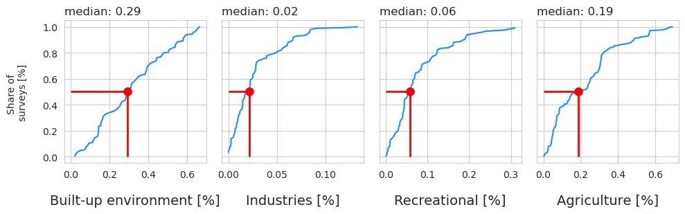
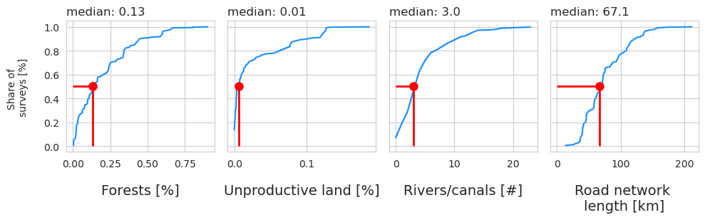
1.3.12. Land use characteristics @ 1500 m#
Show code cell source
fdx = SurveyResults()
df = fdx.surveyResults()
location_no_luse = ["linth_route9brucke",
                "seez_spennwiesenbrucke",
                'limmat_dietikon_keiserp',
                "seez"]

city_no_luse = ["Walenstadt", "Weesen", "Glarus Nord", "Quarten"]

df = df[~df.location.isin(no_luse_data)]
df = df[~df.city.isin(city_no_luse)]

dfdt = df.groupby(["loc_date", "location"], as_index=False).pcs_m.sum()

def applyBufferDataToSurveys(data, buffer_data):

    locations = data.location.unique()


    for location in locations:
        if location in buffer_data.columns:
            landuse = buffer_data[location]
            data.loc[data.location == location, landuse.index] = landuse.values
        else:
            print(location)
            pass
    return data

daily_totals_landuse = applyBufferDataToSurveys(dfdt, buffer_vals)


pretty_names = {"buildings":"Built-up environment [%]",
                'industrial':'Industries [%]',
                'recreation': 'Recreational [%]',
                'agriculture':'Agriculture [%]',
                'woods':'Forests [%]',
                'unproductive':'Unproductive land [%]',
                'roads':'Road network \nlength [km]',
                'intersects': 'Rivers/canals [#]',
               }

# method to get the ranked correlation of pcs_m to each explanatory variable
def make_plot_with_spearmans(data, ax, n):
    sns.scatterplot(data=data, x=n, y=unit_label, ax=ax, color='black', s=30, edgecolor='white', alpha=0.6)
    corr, a_p = stats.spearmanr(data[n], data[unit_label])
    return ax, corr, a_p

sns.set_style("whitegrid")
fig, axs = plt.subplots(1,4, figsize=(10,3.2), sharey=True)

data = daily_totals_landuse
loi = ['buildings', 'industrial','recreation','agriculture','woods','unproductive', 'intersects', 'roads']
for i, n in enumerate(loi[:4]):
    ax=axs[i]

    # the ECDF of the land use variable
    the_data = ECDF(data[n].values)
    sns.lineplot(x=the_data.x, y= (the_data.y), ax=ax, color='dodgerblue', label="% of surface area" )

    # get the median % of land use for each variable under consideration from the data
    the_median = data[n].median()

    # plot the median and drop horzontal and vertical lines
    ax.scatter([the_median], .5, color='red',s=50, linewidth=2, zorder=100, label="the median")
    ax.vlines(x=the_median, ymin=0, ymax=.5, color='red', linewidth=2)
    ax.hlines(xmax=the_median, xmin=0, y=0.5, color='red', linewidth=2)

    #remove the legend from ax
    ax.get_legend().remove()

    if i == 0:
        ax.set_ylabel("Share of \nsurveys [%]", labelpad = 15)
    else:
        pass

    # add the median value from all locations to the ax title
    ax.set_title(F"median: {(round(the_median, 2))}",fontsize=12, loc='left')
    ax.set_xlabel(pretty_names[n], fontsize=14, labelpad=15)

plt.tight_layout()

plt.show()
1.3.13. Total correlations, total positive correlations, total negative corrrelations for each buffer radius#
Show code cell source
def countTheNumberOfCorrelationsPerBuffer(pvals: pdtype = None, rhovals: pdtype = None) -> (pdtype, pstype):

    # the number of times p <= 0.05
    number_p_less_than = (pvals <= 0.05).sum()
    number_p_less_than.name = "correlated"

    # the number of postive correlations
    number_pos = (rhovals > 0).sum()
    number_pos.name = "positive"

    # the number of negative correlations
    number_neg = (rhovals < 0).sum()
    number_neg.name = "negative"

    ncorrelated = pd.DataFrame([number_p_less_than, number_pos, number_neg])
    ncorrelated["total"] = ncorrelated.sum(axis=1)
    totals = ncorrelated.total


    return ncorrelated, totals

ncorrelated, total = countTheNumberOfCorrelationsPerBuffer(pvals, rhovals)

pairs = [
    (pvals, rhovals, "1.5k"),
    (pvals2k, rhovals2k, "2k"),
    (pvals25k, rhovals25k, "2.5k"),
    (pvals3k, rhovals3k, "3k"),
    (pvals35k, rhovals35k, "3.5k"),
    (pvals4k, rhovals4k, "4k"),
    (pvals45k, rhovals45k, "4.5k"),
    (pvals5k, rhovals5k, "5k"),
    (pvals10k, rhovals10k, "10k")
]

rho_vals_all = [
    rho_at_buffer,
    rho_at_2k,
    rho_at_25k,
    rho_at_3k,
    rho_at_35k,
    rho_at_4k,
    rho_at_45k,
    rho_at_5k,
    rho_at_10k
]

buffers = [
    new_buffer,
    new_buffer_2k,
    new_buffer_2_5k,
    new_buffer_3k,
    new_buffer_3_5k,
    new_buffer_4k,
    new_buffer_4_5k,
    new_buffer_5k,
    new_buffer_10k
]

rhos_and_ps = []
for pair in pairs:
    _, total = countTheNumberOfCorrelationsPerBuffer(pair[0], pair[1])
    total.name = pair[2]
    rhos_and_ps.append(total)

correlation_results = pd.DataFrame(rhos_and_ps)

res = correlation_results.style.set_table_styles(table_css_styles)
res
| correlated | positive | negative | |
|---|---|---|---|
| 1.5k | 106 | 53 | 53 |
| 2k | 102 | 53 | 49 |
| 2.5k | 103 | 50 | 53 |
| 3k | 97 | 48 | 49 |
| 3.5k | 98 | 50 | 48 |
| 4k | 95 | 49 | 46 |
| 4.5k | 93 | 49 | 44 |
| 5k | 95 | 49 | 46 |
| 10k | 81 | 52 | 29 |
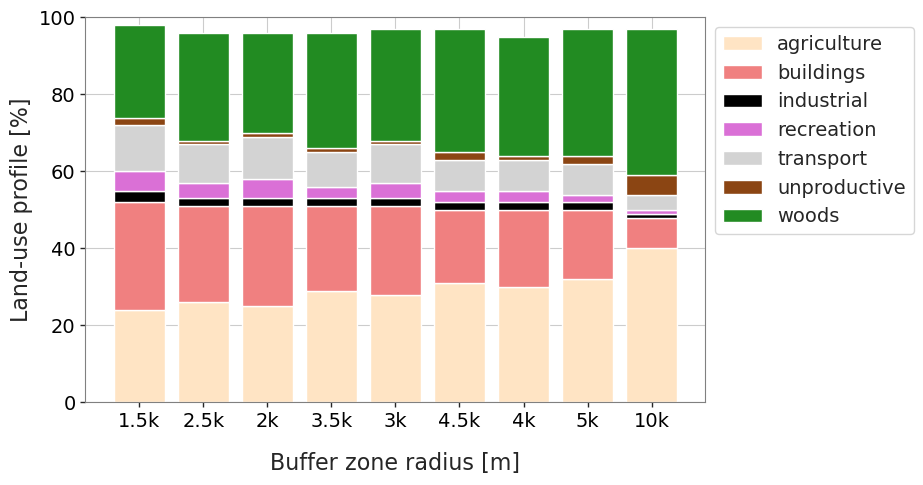
1.3.14. Changes of land use profile for different buffer zones#
As the radius of the buffer zone changes the land use mix changes. Defining the radius of the buffer zone is determined by the scale at which the reporting is being done. For the report to Switzerland the target administrative level was the municipality. Therefore a radius of 1500m was appropriate, given the geographic size of a municipality in Switzerland.
Show code cell source
def combineAdjustedBuffers(buffers, pairs):

    combined_buffers = []
    for i,n in enumerate(pairs):
        a_buffer=buffers[i].adjusted_buffer
        a_buffer["radius"] = n[2]
        combined_buffers.append(a_buffer[["label", "radius"]])

    return pd.concat(combined_buffers, axis=0)
combined_buffers = combineAdjustedBuffers(buffers, pairs)

total_radius = combined_buffers.groupby("radius", as_index=False).label.value_counts()

total_radius = total_radius[total_radius.label != "water"]
total_radius = total_radius.pivot(index="radius", columns="label")
total_radius.columns = total_radius.columns.droplevel()
total_radius = total_radius.div(total_radius.sum(axis=1), axis=0).T
total_radius = total_radius[[total_radius.columns[0], *total_radius.columns[2:], total_radius.columns[1]]]
total_radius = total_radius.mul(100).astype(int)
total_radius.columns.name = None
total_radius.index.name = None
total_radius.style.set_table_styles(table_css_styles)
| 1.5k | 2.5k | 2k | 3.5k | 3k | 4.5k | 4k | 5k | 10k | |
|---|---|---|---|---|---|---|---|---|---|
| agriculture | 24 | 26 | 25 | 29 | 28 | 31 | 30 | 32 | 40 |
| buildings | 28 | 25 | 26 | 22 | 23 | 19 | 20 | 18 | 8 |
| industrial | 3 | 2 | 2 | 2 | 2 | 2 | 2 | 2 | 1 |
| recreation | 5 | 4 | 5 | 3 | 4 | 3 | 3 | 2 | 1 |
| transport | 12 | 10 | 11 | 9 | 10 | 8 | 8 | 8 | 4 |
| unproductive | 2 | 1 | 1 | 1 | 1 | 2 | 1 | 2 | 5 |
| woods | 24 | 28 | 26 | 30 | 29 | 32 | 31 | 33 | 38 |
Below: Chart of different land use profiles at different buffer radiuses
Show code cell source
data =total_radius.values
labels = total_radius.index
colors = total_radius.index
xlabels = [str(x) for x in total_radius.columns]

colors = ['bisque','lightcoral','k','orchid','lightgrey','saddlebrown', 'forestgreen']

bottom = [0]*(len(total_radius.columns))

width = 0.8      # the width of the bars: can also be len(x) sequence

fig, ax = plt.subplots(figsize=(8,5))

for i,group in enumerate(data):
    ax.bar(xlabels, group, width, bottom=bottom, label=labels[i], color = colors[i])
    bottom += group


ax.set_ylabel('Land-use profile [%]', fontsize=16)

ax.set_xlabel("Buffer zone radius [m]", labelpad =15, fontsize=16)
ax.set_facecolor('white')

ax.spines['top'].set_color('0.5')
ax.spines['right'].set_color('0.5')
ax.spines['bottom'].set_color('0.5')
ax.spines['left'].set_color('0.5')
ax.set_ylim(0,100)

ax.xaxis.set_ticks_position('bottom')
ax.yaxis.set_ticks_position('left')
ax.tick_params(labelcolor='k', labelsize=14, width=1)

ax.legend(bbox_to_anchor=(1,1), facecolor = 'white', fontsize=14)

plt.show()
1.3.15. Sum of the total number of objects with a correlation (positive or negative) collected under the different land use categories#
Show code cell source
def numberOfObjectsCorrelatedPerAttribute(rho_at_buffer: pdtype = None, df: pdtype = None) -> pdtype:

    # select all the codes that have a p-value less than 0.05
    p_less_than = rho_at_buffer[rho_at_buffer.exact_p <= 0.05]

    # group the codes by land use attribute
    p_less_than_use_codes = p_less_than.groupby("use").code.unique()

    # sume the number of objects with a correlation (positive or negative) for each land use attribute
    results = nObjectsPerLandUse(p_less_than_use_codes,df)

    return results

numberOfObjectsCorrelatedPerAttribute(rho_at_buffer, df)
| total | |
|---|---|
| agriculture | 22736 |
| buildings | 16004 |
| industrial | 14762 |
| intersects | 21301 |
| recreation | 26231 |
| roads | 17108 |
| unproductive | 20865 |
| woods | 14104 |
1.3.16. The % total of materials of the objects of interest with respect to the total number of objects collected.#
Show code cell source
def thePercentTotalOfMaterials(codes, df, materialmap):

    total = df.quantity.sum()
    buffer_codes = df[df.code.isin(codes)].copy()
    buffer_codes["material"] = buffer_codes.code.apply(lambda x: materialmap[x])

    material_df = pd.DataFrame(buffer_codes.groupby("material").quantity.sum()/total).round(3)

    material_df["quantity"] = material_df.quantity.apply(lambda x: f'{int((x*100))}%')

    return material_df

thePercentTotalOfMaterials(codes_fail, df, code_m_map)
| quantity | |
|---|---|
| material | |
| Cloth | 0% |
| Glass | 5% |
| Metal | 2% |
| Paper | 1% |
| Plastic | 75% |
1.3.17. The % total of the objects of interest with respect to all objects collected.#
Show code cell source
def thePercentTotalOfTheTopXObjects(df, codes):
    index = [f'ratio of the items of interest over all items:',f'number of items of interest:']
    item_totals = df.groupby("code").quantity.sum().sort_values(ascending=False)
    top_x = item_totals.loc[codes].sum()
    total = df.quantity.sum()
    data = [f"{(round((top_x /total)*100))}%","{:,}".format(round(top_x))]
    return pd.DataFrame(data=data, index=index, columns=["value"])

thePercentTotalOfTheTopXObjects(df,codes_fail)
| value | |
|---|---|
| ratio of the items of interest over all items: | 84% |
| number of items of interest: | 39,442 |
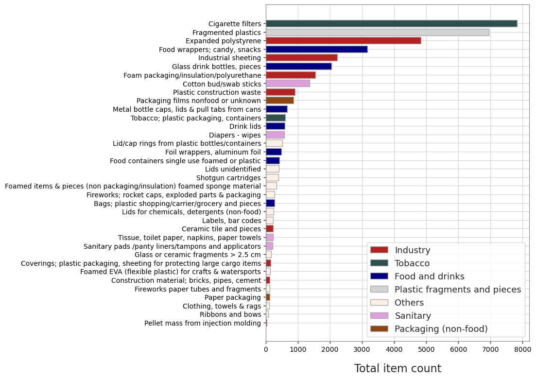
1.3.18. The cumulative totals of the objects of interest, grouped by economic source#
The object of interest were grouped according to economic source by considering the possible uses for each object, as defined in the object description and sources columns of the default codes data:
tobaco: “Tobacco”, “Smoking related”
industry: ‘Industry’,’Construction’, ‘Industrial’, ‘Manufacturing’
sanitary: “Sanitary”, “Personal hygiene”, “Water treatment”
packaging: ‘Packaging (non-food)’,’Packaging films nonfood or unknown’, ‘Paper packaging’
food: ‘Food and drinks’,’Foil wrappers, aluminum foil’, ‘Food and drinks’, ‘Food and drink’
fragments: ‘Plastic fragments and pieces’, ‘Plastic fragments angular <5mm’, ‘Styrofoam < 5mm’, ‘Plastic fragments rounded <5mm’, ‘Foamed plastic <5mm’, ‘Fragmented plastics’
Show code cell source
def check_condition(x, conditions, i):

    if list(set(x)&set(conditions[i])):
        data = conditions[i][0]
    elif i == 0 and not list(set(x)&set(conditions[i])):
        data = "Others"
    else:
        data = check_condition(x, conditions, i-1)
    return data

# define the broad categories:
tobaco = ["Tobacco", "Smoking related"]
industry = ['Industry','Construction', 'Industrial', 'Manufacturing']
sanitary = ["Sanitary", "Personal hygiene", "Water treatment"]
packaging = ['Packaging (non-food)','Packaging films nonfood or unknown', 'Paper packaging']
food = ['Food and drinks','Foil wrappers, aluminum foil', 'Food and drinks', 'Food and drink']
fragments = ['Plastic fragments and pieces',
             'Plastic fragments angular <5mm',
             'Styrofoam < 5mm',
             'Plastic fragments rounded <5mm',
             'Foamed  plastic <5mm',
             'Fragmented plastics',
            ]

conditions = [tobaco, industry, sanitary, packaging, food, fragments]


dT20 = df[df.code.isin(codes_fail)].groupby("code", as_index=False).quantity.sum().sort_values("quantity", ascending=False)
dT20["description"] = dT20.code.map(lambda x: code_d_map[x])
dT20.set_index("code", drop=True, inplace=True)


for each_code in dT20.index:
    srcs = dfCodes.loc[each_code][["source", "source_two", "source_three", "description"]]
    a = check_condition(srcs.values, conditions, len(conditions)-1)
    dT20.loc[each_code, "Type"] = a

total_type = dT20.groupby(["Type"], as_index=False).quantity.sum()
total_type["Proportion [%]"] = ((total_type.quantity/df.quantity.sum())*100).round(1)
total_type.style.format(precision=1).set_table_styles(table_css_styles)
| Type | quantity | Proportion [%] | |
|---|---|---|---|
| 0 | Food and drinks | 7652 | 16.3 |
| 1 | Industry | 10060 | 21.5 |
| 2 | Others | 3001 | 6.4 |
| 3 | Packaging (non-food) | 971 | 2.1 |
| 4 | Plastic fragments and pieces | 6943 | 14.8 |
| 5 | Sanitary | 2381 | 5.1 |
| 6 | Tobacco | 8434 | 18.0 |
Show code cell source
fig, ax = plt.subplots(figsize=(7,9))
colors = {'Industry': 'firebrick', 'Tobacco': 'darkslategrey', 'Food and drinks': 'navy', 'Plastic fragments and pieces':'lightgrey',
         'Others':'linen','Sanitary':'plum','Packaging (non-food)':'saddlebrown'}

width = 0.6

labels = list(colors.keys())
handles = [plt.Rectangle((0,0),1,1, color=colors[label]) for label in labels]

ax.barh(dT20.description, dT20.quantity, color=[colors[i] for i in dT20.Type], edgecolor='darkgrey')
ax.invert_yaxis()
ax.set_ylabel('')
xticks = [0,1000, 2000, 3000, 4000, 5000, 6000, 7000, 8000]
ax.set_xticks(xticks)
ax.set_xticklabels([str(x) for x in xticks])


ax.set_xlabel('Total item count', fontsize=16, labelpad =15)
ax.xaxis.set_ticks_position('bottom')
ax.yaxis.set_ticks_position('left')
ax.tick_params(labelcolor='k', labelsize=10, width=1)
ax.yaxis.grid(color='lightgray')
ax.xaxis.grid(color='lightgray')
ax.set_facecolor('white')

plt.legend(handles, labels, fontsize=13,facecolor='white', loc="lower right")
for ha in ax.legend_.legend_handles:
    ha.set_edgecolor("darkgrey")

plt.grid(True)
ax.spines['top'].set_color('0.5')
ax.spines['right'].set_color('0.5')
ax.spines['bottom'].set_color('0.5')
ax.spines['left'].set_color('0.5')

# plt.savefig('C:/Users/schre086/figures/land_use_ch/top_20items.png', bbox_inches='tight')

plt.show()
1.3.18.1. Litter items of local origin#
Items that have four or more positive associations with a land use category.
Show code cell source
correlated = rho_at_buffer[(rho_at_buffer.exact_p <= 0.05) & (rho_at_buffer.rho > 0)]
local = correlated.code.value_counts()
local = local[local >= 4]
local.name = "correlations"
quantity = df[df.code.isin(local.index)].groupby("code").quantity.sum()
items_of_local_origin = pd.DataFrame([local, quantity]).T
items_of_local_origin
| correlations | quantity | |
|---|---|---|
| code | ||
| G27 | 4 | 7821 |
| G904 | 4 | 279 |
| G177 | 4 | 482 |
1.3.18.2. Ubiquitous items#
Items that have three or less positive associations with a land use category and are positively associated with river or stream intersections.
Show code cell source
correlated = rho_at_buffer[(rho_at_buffer.exact_p <= 0.05) & (rho_at_buffer.rho > 0)]
pos_intersects = rho_at_buffer[(rho_at_buffer.use == "intersects") & (rho_at_buffer.exact_p <= 0.05)]
correlated = correlated[correlated.code.isin(pos_intersects.code.unique())]
local = correlated.code.value_counts()
local = local[local <= 3]
local.name = "correlations"
quantity = df[df.code.isin(local.index)].groupby("code").quantity.sum()
items_of_local_origin = pd.DataFrame([local, quantity]).T
items_of_local_origin
| correlations | quantity | |
|---|---|---|
| code | ||
| G98 | 3 | 581 |
| G941 | 3 | 857 |
| G178 | 3 | 668 |
| G25 | 3 | 613 |
| G21 | 2 | 593 |
| G23 | 2 | 405 |
| Gfrags | 2 | 6943 |
| G74 | 2 | 1546 |
| G67 | 1 | 2221 |
| G10 | 1 | 422 |
| G89 | 1 | 916 |
| G70 | 1 | 390 |
| G944 | 1 | 34 |
| Gfoam | 1 | 4833 |
1.3.18.3. Other items#
Items that have three or less positive associations with a land use category and are NOT positively associated with river or stream intersections.
Show code cell source
correlated = rho_at_buffer[(rho_at_buffer.exact_p <= 0.05) & (rho_at_buffer.rho > 0)]
pos_intersects = rho_at_buffer[(rho_at_buffer.use == "intersects") & (rho_at_buffer.exact_p > 0.05)]
correlated = correlated[correlated.code.isin(pos_intersects.code.unique())]
local = correlated.code.value_counts()
local = local[local <= 3]
local.name = "correlations"
quantity = df[df.code.isin(local.index)].groupby("code").quantity.sum()
items_of_local_origin = pd.DataFrame([local, quantity]).T
items_of_local_origin
| correlations | quantity | |
|---|---|---|
| code | ||
| G30 | 3 | 3159 |
| G923 | 3 | 223 |
| G3 | 2 | 277 |
| G24 | 2 | 509 |
| G200 | 1 | 2051 |
| G95 | 1 | 1369 |
| G208 | 1 | 165 |
| G940 | 1 | 131 |
| G922 | 1 | 233 |
1.4. Annex#
Land-use attributes of the survey locations.
Show code cell source
results = buffer_vals.T.round(3)
display_columns = ["buildings",  "industrial", "roads", "recreation", "agriculture","woods", "intersects", "unproductive"]

res = results[display_columns].style.format(precision=3).set_table_styles(table_css_styles)

glue("all_luse", res, display=False)
| label | buildings | industrial | roads | recreation | agriculture | woods | intersects | unproductive |
|---|---|---|---|---|---|---|---|---|
| maladaire | 0.509 | 0.015 | 75.300 | 0.044 | 0.238 | 0.032 | 3.000 | 0.000 |
| preverenges | 0.294 | 0.084 | 67.100 | 0.065 | 0.305 | 0.078 | 2.000 | 0.003 |
| caprino | 0.046 | 0.000 | 14.900 | 0.003 | 0.020 | 0.904 | 14.000 | 0.013 |
| foce-del-cassarate | 0.631 | 0.005 | 86.200 | 0.081 | 0.005 | 0.049 | 5.000 | 0.000 |
| lido | 0.632 | 0.006 | 83.300 | 0.084 | 0.006 | 0.048 | 5.000 | 0.000 |
| lugano-centro | 0.636 | 0.017 | 105.700 | 0.059 | 0.025 | 0.042 | 5.000 | 0.000 |
| spiaggia-parco-ciani | 0.629 | 0.005 | 87.600 | 0.080 | 0.005 | 0.051 | 5.000 | 0.000 |
| via-brunari-spiaggia | 0.283 | 0.021 | 116.400 | 0.059 | 0.086 | 0.410 | 0.000 | 0.009 |
| golene-gudo | 0.078 | 0.001 | 74.500 | 0.006 | 0.558 | 0.315 | 0.000 | 0.018 |
| isole-di-brissago-porto | 0.365 | 0.000 | 13.200 | 0.054 | 0.014 | 0.473 | 9.000 | 0.000 |
| magadino-lido | 0.100 | 0.005 | 41.300 | 0.005 | 0.128 | 0.585 | 23.000 | 0.123 |
| rivapiana | 0.580 | 0.018 | 87.700 | 0.093 | 0.039 | 0.137 | 7.000 | 0.000 |
| via-mirasole-spiaggia | 0.312 | 0.022 | 121.700 | 0.065 | 0.084 | 0.378 | 0.000 | 0.007 |
| aare-port | 0.233 | 0.063 | 120.300 | 0.063 | 0.185 | 0.379 | 0.000 | 0.001 |
| schutzenmatte | 0.265 | 0.029 | 117.500 | 0.023 | 0.263 | 0.336 | 0.000 | 0.003 |
| zugerseecholler_cham_blarerm | 0.250 | 0.121 | 64.600 | 0.057 | 0.325 | 0.020 | 8.000 | 0.040 |
| la-petite-plage | 0.335 | 0.040 | 72.100 | 0.123 | 0.144 | 0.109 | 5.000 | 0.079 |
| vidy-ruines | 0.312 | 0.066 | 99.600 | 0.309 | 0.066 | 0.018 | 2.000 | 0.000 |
| baby-plage-geneva | 0.540 | 0.007 | 136.100 | 0.161 | 0.045 | 0.022 | 2.000 | 0.000 |
| grand-clos | 0.164 | 0.012 | 39.700 | 0.044 | 0.070 | 0.599 | 8.000 | 0.020 |
| weissenau-neuhaus | 0.027 | 0.015 | 46.200 | 0.189 | 0.311 | 0.337 | 13.000 | 0.077 |
| evole-plage | 0.396 | 0.023 | 113.900 | 0.085 | 0.025 | 0.238 | 1.000 | 0.003 |
| oberi-chlihochstetten | 0.124 | 0.031 | 75.200 | 0.009 | 0.505 | 0.229 | 0.000 | 0.037 |
| plage-de-serriere | 0.408 | 0.053 | 103.500 | 0.056 | 0.028 | 0.233 | 2.000 | 0.000 |
| vierwaldstattersee_weggis_schoberls_1 | 0.145 | 0.012 | 44.300 | 0.005 | 0.672 | 0.123 | 5.000 | 0.000 |
| vierwaldstattersee_weggis_schoberls_2 | 0.140 | 0.013 | 43.700 | 0.005 | 0.679 | 0.122 | 5.000 | 0.000 |
| vierwaldstattersee_weggis_schoberls_3 | 0.207 | 0.014 | 34.700 | 0.014 | 0.571 | 0.136 | 4.000 | 0.000 |
| mullermatte | 0.258 | 0.022 | 109.600 | 0.069 | 0.084 | 0.435 | 3.000 | 0.007 |
| limmat_unterengstringen_oggierbuhrer | 0.310 | 0.092 | 125.800 | 0.035 | 0.306 | 0.106 | 0.000 | 0.003 |
| limmat_zuerich_wagnerc | 0.385 | 0.079 | 144.500 | 0.130 | 0.130 | 0.120 | 0.000 | 0.000 |
| limmat_zurich_mortensena_meiera | 0.442 | 0.051 | 153.200 | 0.149 | 0.088 | 0.079 | 0.000 | 0.000 |
| quai-maria-belgia | 0.582 | 0.028 | 72.600 | 0.060 | 0.043 | 0.021 | 4.000 | 0.000 |
| sihl_zuerich_eggerskoehlingera | 0.601 | 0.015 | 173.900 | 0.066 | 0.001 | 0.015 | 0.000 | 0.000 |
| bielersee_vinelz_fankhausers | 0.155 | 0.008 | 58.500 | 0.034 | 0.568 | 0.134 | 5.000 | 0.063 |
| erlach-camping-strand | 0.136 | 0.011 | 38.800 | 0.057 | 0.430 | 0.186 | 7.000 | 0.133 |
| anarchy-beach | 0.665 | 0.009 | 48.500 | 0.052 | 0.061 | 0.004 | 3.000 | 0.000 |
| rastplatz-stampf | 0.284 | 0.060 | 40.200 | 0.108 | 0.297 | 0.004 | 10.000 | 0.121 |
| zuerichsee_richterswil_benkoem_2 | 0.389 | 0.017 | 61.800 | 0.040 | 0.248 | 0.164 | 3.000 | 0.000 |
| sentiero-giro-del-golf-spiaggia | 0.311 | 0.000 | 26.700 | 0.286 | 0.252 | 0.063 | 3.000 | 0.029 |
| vira-gambarogno | 0.174 | 0.003 | 41.500 | 0.003 | 0.066 | 0.660 | 18.000 | 0.006 |
| canale-saleggi | 0.304 | 0.021 | 120.200 | 0.061 | 0.089 | 0.383 | 0.000 | 0.009 |
| gummligrabbe | 0.046 | 0.002 | 59.000 | 0.002 | 0.522 | 0.354 | 0.000 | 0.054 |
| mannewil | 0.039 | 0.002 | 68.300 | 0.000 | 0.461 | 0.461 | 0.000 | 0.017 |
| lavey-les-bains-2 | 0.208 | 0.033 | 93.000 | 0.019 | 0.186 | 0.397 | 0.000 | 0.035 |
| schusspark-strand | 0.384 | 0.085 | 140.800 | 0.069 | 0.057 | 0.228 | 0.000 | 0.001 |
| pfafikon-bad | 0.273 | 0.086 | 62.600 | 0.024 | 0.252 | 0.099 | 6.000 | 0.110 |
| zurichsee_kusnachterhorn_thirkell-whitej | 0.651 | 0.010 | 57.800 | 0.042 | 0.072 | 0.098 | 3.000 | 0.003 |
| plage-de-cheyres | 0.143 | 0.003 | 36.300 | 0.030 | 0.309 | 0.342 | 4.000 | 0.127 |
| leuk-mattenstrasse | 0.112 | 0.002 | 87.200 | 0.014 | 0.189 | 0.514 | 0.000 | 0.106 |
| thun-strandbad | 0.627 | 0.055 | 97.200 | 0.089 | 0.055 | 0.026 | 4.000 | 0.002 |
| zurichsee_wollishofen_langendorfm | 0.441 | 0.028 | 94.600 | 0.195 | 0.051 | 0.036 | 1.000 | 0.013 |
| pont-sous-terre | 0.477 | 0.071 | 212.000 | 0.117 | 0.012 | 0.047 | 0.000 | 0.002 |
| oben-am-see | 0.117 | 0.030 | 58.300 | 0.024 | 0.324 | 0.421 | 12.000 | 0.016 |
| thunersee_spiez_meierd_1 | 0.142 | 0.025 | 45.800 | 0.009 | 0.481 | 0.245 | 3.000 | 0.009 |
| cully-plage | 0.087 | 0.002 | 62.800 | 0.005 | 0.638 | 0.135 | 11.000 | 0.002 |
| preverenges-le-sout | 0.318 | 0.066 | 55.000 | 0.079 | 0.325 | 0.103 | 1.000 | 0.003 |
| la-pecherie | 0.091 | 0.023 | 41.400 | 0.005 | 0.665 | 0.146 | 3.000 | 0.005 |
| villa-barton | 0.467 | 0.006 | 85.100 | 0.230 | 0.021 | 0.015 | 0.000 | 0.000 |
| zurcher-strand | 0.561 | 0.009 | 156.600 | 0.129 | 0.005 | 0.009 | 3.000 | 0.000 |
| oyonne | 0.631 | 0.016 | 97.300 | 0.045 | 0.061 | 0.024 | 2.000 | 0.000 |
| lavey-la-source | 0.091 | 0.029 | 83.900 | 0.010 | 0.136 | 0.620 | 0.000 | 0.019 |
| lavey-les-bains | 0.178 | 0.032 | 89.600 | 0.016 | 0.182 | 0.445 | 0.000 | 0.032 |
| spackmatt | 0.229 | 0.022 | 96.400 | 0.040 | 0.342 | 0.289 | 0.000 | 0.001 |
| luscherz-plage | 0.079 | 0.000 | 37.300 | 0.009 | 0.269 | 0.601 | 6.000 | 0.015 |
| strandboden-biel | 0.346 | 0.025 | 124.400 | 0.079 | 0.048 | 0.341 | 3.000 | 0.007 |
| jona-river-rastplatz | 0.304 | 0.062 | 45.600 | 0.104 | 0.277 | 0.004 | 11.000 | 0.127 |
| reuss_hunenberg_eberhardy | 0.059 | 0.005 | 66.000 | 0.002 | 0.668 | 0.042 | 0.000 | 0.186 |
| reuss_ottenbach_schoenenbergerl | 0.114 | 0.011 | 73.400 | 0.005 | 0.650 | 0.082 | 0.000 | 0.094 |
| zuerichsee_staefa_hennm | 0.242 | 0.011 | 51.400 | 0.006 | 0.489 | 0.163 | 4.000 | 0.017 |
| signalpain | 0.411 | 0.068 | 83.900 | 0.124 | 0.036 | 0.099 | 7.000 | 0.056 |
| baby-plage-ii-geneve | 0.549 | 0.007 | 132.200 | 0.162 | 0.053 | 0.023 | 2.000 | 0.000 |
| pointe-dareuse | 0.143 | 0.056 | 32.300 | 0.012 | 0.563 | 0.163 | 8.000 | 0.004 |
| les-glariers | 0.078 | 0.014 | 107.000 | 0.009 | 0.546 | 0.207 | 0.000 | 0.036 |
| nidau-strand | 0.383 | 0.040 | 119.600 | 0.099 | 0.099 | 0.200 | 3.000 | 0.008 |
| tiger-duck-beach | 0.357 | 0.035 | 105.300 | 0.239 | 0.130 | 0.063 | 1.000 | 0.002 |
| zuerichsee_waedenswil_colomboc_1 | 0.346 | 0.014 | 68.000 | 0.046 | 0.320 | 0.157 | 3.000 | 0.000 |
| camp-des-peches | 0.168 | 0.024 | 74.200 | 0.053 | 0.513 | 0.141 | 8.000 | 0.004 |
| delta-park | 0.213 | 0.074 | 56.700 | 0.016 | 0.279 | 0.240 | 5.000 | 0.049 |
| le-pierrier | 0.539 | 0.027 | 62.700 | 0.072 | 0.154 | 0.031 | 4.000 | 0.000 |
| pecos-plage | 0.155 | 0.030 | 59.800 | 0.045 | 0.565 | 0.096 | 6.000 | 0.011 |
| beich | 0.021 | 0.003 | 67.100 | 0.003 | 0.692 | 0.215 | 0.000 | 0.033 |
| aare_suhrespitz_badert | 0.298 | 0.067 | 132.800 | 0.038 | 0.259 | 0.227 | 0.000 | 0.006 |
| tschilljus | 0.086 | 0.014 | 83.400 | 0.027 | 0.356 | 0.420 | 0.000 | 0.037 |
| sundbach-strand | 0.076 | 0.000 | 40.400 | 0.021 | 0.217 | 0.645 | 9.000 | 0.003 |
| wycheley | 0.074 | 0.027 | 50.800 | 0.017 | 0.291 | 0.517 | 12.000 | 0.016 |
| aare_koniz_hoppej | 0.466 | 0.010 | 157.200 | 0.088 | 0.133 | 0.151 | 0.000 | 0.003 |
| camping-gwatt-strand | 0.297 | 0.088 | 66.500 | 0.069 | 0.230 | 0.145 | 6.000 | 0.044 |
| bern-tiergarten | 0.451 | 0.010 | 152.300 | 0.086 | 0.131 | 0.179 | 0.000 | 0.004 |
| boiron | 0.183 | 0.079 | 35.600 | 0.029 | 0.412 | 0.167 | 1.000 | 0.000 |
| rocky-plage | 0.533 | 0.007 | 126.900 | 0.167 | 0.057 | 0.024 | 2.000 | 0.000 |
| lacleman_gland_lecoanets | 0.123 | 0.005 | 42.800 | 0.123 | 0.378 | 0.332 | 0.000 | 0.000 |
| route-13 | 0.467 | 0.037 | 131.800 | 0.119 | 0.112 | 0.107 | 1.000 | 0.003 |
| schmerikon-bahnhof-strand | 0.119 | 0.056 | 76.000 | 0.022 | 0.381 | 0.241 | 12.000 | 0.101 |
| aabach | 0.121 | 0.050 | 65.300 | 0.026 | 0.255 | 0.384 | 16.000 | 0.119 |
| la-thiele_le-mujon_confluence | 0.318 | 0.050 | 116.200 | 0.060 | 0.405 | 0.012 | 0.000 | 0.001 |
| nouvelle-plage | 0.280 | 0.050 | 52.600 | 0.073 | 0.335 | 0.090 | 4.000 | 0.090 |
| baye-de-montreux-g | 0.476 | 0.000 | 70.700 | 0.052 | 0.111 | 0.129 | 3.000 | 0.000 |
| les-vieux-ronquoz | 0.241 | 0.133 | 138.000 | 0.036 | 0.188 | 0.187 | 0.000 | 0.013 |
| sihl_zuerich_eichenbergerd | 0.237 | 0.007 | 124.300 | 0.068 | 0.130 | 0.420 | 0.000 | 0.014 |
| versoix | 0.592 | 0.022 | 66.800 | 0.049 | 0.140 | 0.063 | 5.000 | 0.003 |
| augustmutzenbergstrandweg | 0.361 | 0.010 | 78.700 | 0.032 | 0.271 | 0.195 | 0.000 | 0.005 |
| parc-des-pierrettes | 0.468 | 0.008 | 84.400 | 0.177 | 0.124 | 0.056 | 1.000 | 0.000 |
| plage-de-st-sulpice | 0.494 | 0.014 | 73.000 | 0.163 | 0.157 | 0.057 | 1.000 | 0.000 |
| aare_bern_gerberm | 0.277 | 0.025 | 112.300 | 0.021 | 0.375 | 0.204 | 0.000 | 0.001 |
| brugg-be-buren-bsg-standort | 0.196 | 0.048 | 108.800 | 0.045 | 0.346 | 0.292 | 0.000 | 0.001 |
| kusnachter-dorfbach-tobelweg-1-4 | 0.504 | 0.007 | 96.500 | 0.033 | 0.139 | 0.219 | 3.000 | 0.004 |
| ruisseau-de-la-croix-plage | 0.118 | 0.003 | 32.200 | 0.032 | 0.339 | 0.385 | 5.000 | 0.078 |
| ligerz-strand | 0.118 | 0.000 | 50.800 | 0.018 | 0.366 | 0.416 | 3.000 | 0.029 |
| hafeli | 0.190 | 0.055 | 70.300 | 0.021 | 0.352 | 0.286 | 6.000 | 0.005 |
| aare-solothurn-lido-strand | 0.133 | 0.024 | 86.300 | 0.027 | 0.400 | 0.289 | 0.000 | 0.002 |
| bern-fahrstrasse | 0.253 | 0.030 | 135.600 | 0.047 | 0.192 | 0.362 | 0.000 | 0.003 |
| gals-reserve | 0.113 | 0.009 | 58.500 | 0.055 | 0.443 | 0.300 | 7.000 | 0.028 |
| ascona-traghetto-spiaggia | 0.447 | 0.024 | 79.400 | 0.116 | 0.049 | 0.218 | 2.000 | 0.004 |
| pacha-mama-gerra | 0.138 | 0.000 | 28.400 | 0.000 | 0.003 | 0.807 | 17.000 | 0.003 |
| gerra-gambarogno | 0.132 | 0.000 | 32.600 | 0.000 | 0.011 | 0.807 | 17.000 | 0.006 |
| san-nazzaro-gambarogno | 0.242 | 0.003 | 45.700 | 0.003 | 0.026 | 0.667 | 13.000 | 0.003 |
| hauterive-petite-plage | 0.279 | 0.048 | 85.200 | 0.099 | 0.189 | 0.243 | 2.000 | 0.013 |
| aare-limmatspitz | 0.169 | 0.055 | 111.900 | 0.013 | 0.316 | 0.323 | 0.000 | 0.003 |
| aare_brugg_buchie | 0.222 | 0.067 | 120.300 | 0.033 | 0.240 | 0.302 | 0.000 | 0.008 |
| bain-des-dames | 0.644 | 0.013 | 65.400 | 0.046 | 0.092 | 0.013 | 2.000 | 0.000 |
| luscherz-two | 0.069 | 0.000 | 39.700 | 0.008 | 0.271 | 0.613 | 6.000 | 0.014 |
| impromptu_cudrefin | 0.113 | 0.005 | 36.100 | 0.038 | 0.523 | 0.190 | 5.000 | 0.100 |
| vira-spiaggia-left-of-river | 0.167 | 0.003 | 42.300 | 0.003 | 0.067 | 0.669 | 18.000 | 0.008 |
| tolochenaz | 0.241 | 0.065 | 63.900 | 0.078 | 0.346 | 0.108 | 2.000 | 0.000 |
| limmat_zuerich_suterdglauserp | 0.409 | 0.068 | 145.700 | 0.087 | 0.052 | 0.130 | 0.000 | 0.000 |
| aare_post | 0.223 | 0.062 | 118.700 | 0.062 | 0.194 | 0.386 | 0.000 | 0.001 |
| aare_bern_scheurerk | 0.323 | 0.081 | 167.200 | 0.065 | 0.072 | 0.256 | 0.000 | 0.002 |
| strandbeiz | 0.297 | 0.064 | 45.200 | 0.112 | 0.273 | 0.004 | 9.000 | 0.104 |
Fig. 1.5 #
figure 1.5: The land use attributes of the survey locations @ 1 500 m radius
This script updated 09/08/2023 in Biel, CH
❤️ what you do everyday
analyst at hammerdirt
Git repo: https://github.com/hammerdirt-analyst/landuse.git

Git branch: main

json      : 2.0.9
seaborn   : 0.12.2
matplotlib: 3.7.1
pandas    : 2.0.0
numpy     : 1.24.2
PIL       : 9.5.0
scipy     : 1.10.1
IPython   : 8.12.0