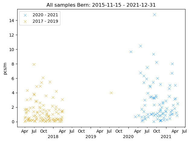
Canton Bern

Density of trash along lakes and rivers

This is a sample cantonal report. The structure and the format are based off of the federal report, (IQAASL). This version is intended for use as a decsion support tool. Thus, the user is expected to be familiar with the results in the federal report and the methods described in the Guide for Monitoring Marine Litter on European Seas (The guide).

Initial assessment: stakeholder discussion and priorities.

Stakeholders should consider the following questions while consulting the report:

1. Are the major rivers and lakes included?

2. Was their more or less observed in 2021 vs the prior results?

3. How do these results compare to assessments from other sources (EAWAG, EMPA, Internal reports)?

   • This includes reports from NGOS in the region

   • Is the data comparable?

4. Are the objects identified as the most common currently the focus of reduction or prevention campaigns?

   • How does the canton decide priorties in this regard?

   • Did or does the object appear in any regional action plan or strategy?

5. For objects that have been the focus of prevention or reduction campaigns in the past: are they on the most common objects list now?

   • If the objects are on the most common list, is this inline with expectations ?

   • What excatly was the mechanism or process that was intended to reduce the presence of the object?

   • With respect to the amount of resources attributed to prevention and mitigation: Do the attributed amounts reflect the importance of the object in terms of total amount found and frequency of occurence?

6. Does the sampling distribution reflect the topography and land-use of the canton?

7. Do the municipalities with elevated pcs/m have common land-use attributes?

8. Are the municipalities of strategic importance to the canton included?

9. Are their locations in the canton that should have been surveyed, according to cantonal priorities?

10. Are their products of regional interest that should be included in the cantonal report?

Map of survey locations

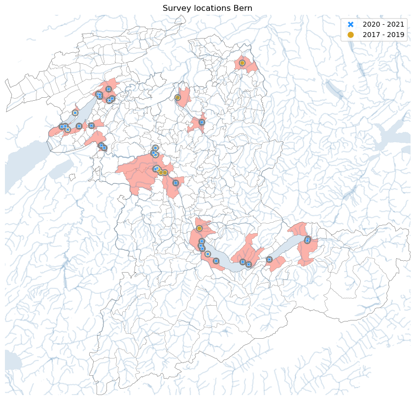
Vital statistics

Use case: Interpret observed values

All data

Features surveyed

• Rivers: 6

• Lakes: 3

Administrative boundaries

• Survey locations: 40

• Cities: 26

Material composition

	% of total
material
cloth	4%
glass	6%
metal	4%
paper	3%
plastic	76%
wood	2%

Survey total pcs/m 2020 - 2021 versus 2017 - 2019. All locations considered.

2017 - 2021

• Number of samples: 195

• Total objects: 13590

• Average pcs/m: 2.01

• Standard deviation: 2.27

• Maximum pcs/m: 14.8

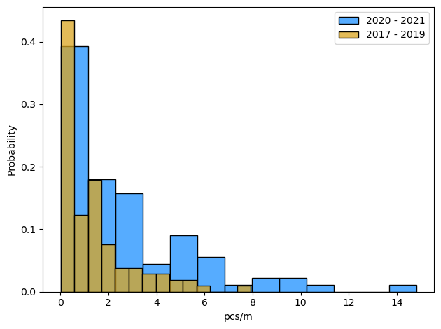
2020 - 2021

• Number of samples: 89

• Total objects: 9028

• Average pcs/m: 2.76

• Standard deviation: 2.74

• Maximum pcs/m: 14.8

2017 - 2019

• Number of samples: 106

• Total objects: 4562

• Average pcs/m: 1.39

• Standard deviation: 1.53

• Maximum pcs/m: 7.92

Lakes

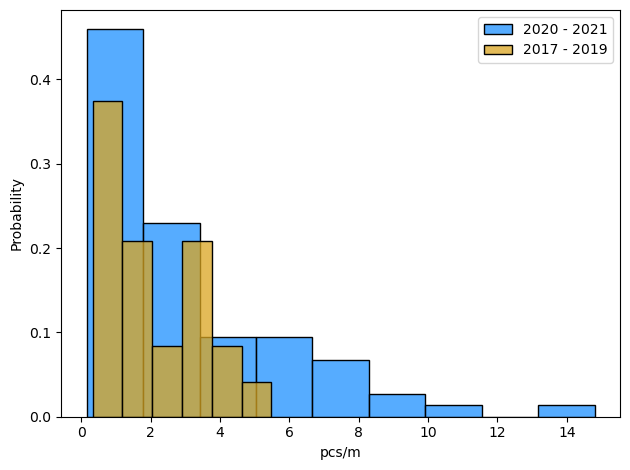
Features surveyed

• Lakes: 3

Administrative boundaries

• Survey locations: 19

• Cities: 13

Material composition

	% of total
material
glass	5%
metal	3%
paper	2%
plastic	84%

Survey total pcs/m 2020 - 2021 v/s 2017 - 2019. All locations considered.

2017 - 2021

• Number of samples: 98

• Total objects: 9889

• Average pcs/m: 2.81

• Standard deviation: 2.63

• Maximum pcs/m: 14.8

2020 - 2021

• Number of samples: 74

• Total objects: 8423

• Average pcs/m: 3.09

• Standard deviation: 2.85

• Maximum pcs/m: 14.8

2017 - 2019

• Number of samples: 24

• Total objects: 1466

• Average pcs/m: 1.96

• Standard deviation: 1.49

• Maximum pcs/m: 5.48

Rivers

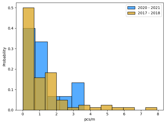
Features surveyed

• Rivers: 6

Administrative boundaries

• Survey locations: 21

• Cities: 14

Material composition

	% of total
material
cloth	15%
glass	7%
metal	10%
paper	6%
plastic	52%
wood	5%

Survey total pcs/m 2020 - 2021 v/s 2017 - 2018. All locations considered.

2017 - 2021

• Number of samples: 97

• Total objects: 3701

• Average pcs/m: 1.21

• Standard deviation: 1.45

• Maximum pcs/m: 7.92

2020 - 2021

• Number of samples: 15

• Total objects: 605

• Average pcs/m: 1.12

• Standard deviation: 1.11

• Maximum pcs/m: 3.63

2017 - 2019

• Number of samples: 82

• Total objects: 3096

• Average pcs/m: 1.22

• Standard deviation: 1.5

• Maximum pcs/m: 7.92

How did we get this data ?

The data is a combination of observations from variety of groups in Switerland since 2015. The observations were recorded using an interpretation of the Guide for Monitoring Marine Litter on European Seas The guide. The guide and the monitoring of beach litter are part of decades of research, here is the brief history A Brief History of Marine Litter Research.

Common sense guidance:

1. The data should be considered as a reasonable estimate of the minimum amount of trash on the ground at the time of the survey.

2. There are many sources of variance. We have considered the following:

   • litter density between sampling groups.

   • litter density with respect to topographical features.

3. There are differences in detect-ability and appearance for items of the same classification that are due to the effects of decomposition.

4. Many surveyors are volunteers and have different levels of experience or physical constraints that limit what will actually be collected and counted.

How to make a report

Survey and Land use

A report is the implementation of a SurveyReport and a LandUseReport. The SurveyReport is the basic element and does the initial aggregating and descriptive statistics for a query.

The land-use-report accepts SurveyReport.sample_results and assigns the land-use attributes to the record. The land-use-report provides the baseline assessment of litter density with reference to the surrounding environment.

The assessment accepts as variables the proportion of available space that a topographical feature occupies in a circle of \(\pi r² \text{ where r = 1 500 meters}\) and the center of that circle is the survey location. These proportions are compared to the average pieces per meter for an object or group of objects.

Create a report

A report can be intiated by providing the name of the canton. If your canton does not appear this is because we have no data. The prior dates will be calculated automatically, by taking all data prior to the start date of the querry.

import reports
import geospatial
import gridforecast

# suppose you have defined your data into df
observed_dates = {'start':'2020-01-01', 'end':'2021-12-31'}

# everything that was seen before
prior_dates = {'start':'2015-11-15', 'end':'2019-12-31'}

# name the canton
canton = 'Bern'

# define the data of interest
data_of_interest = {'canton':canton, 'date_range':observed_dates}

# load the data
df = session_config.collect_survey_data()

# filter the data. 
filtered_data, locations = gridforeacast.filter_data(df, data_of_interest)

# make a survey report
this_report = reports.SurveyReport(dfc=filtered_data)

# generate the parameters for the landuse report
target_df = this_report.sample_results
features = geospatial.collect_topo_data(locations=target_df.location.unique())

# make a landuse report
this_land_use = geospatial.LandUseReport(target_df, features)

Each report and the inference method are documented: SurveyReport, LandUseReport, GridForecaster

Most common objects 2020 - 2021

Use case: Interpret observed values

All data

The most common objects account for 68% of all objects

The most common objects from the selected data. The most common objects are a combination of the top ten most abundant objects and those objects that are found in more than 50% of the samples. Some objects are found frequently but at low quantities.Other objects are found in fewer samples but at higher quantities.

Object	Quantity	pcs/m	% of total	Fail rate
Cigarette filters	1'671	0,42	0,19	0,81
Fragmented plastics	1'323	0,46	0,15	0,89
Industrial sheeting	686	0,24	0,08	0,78
Food wrappers; candy, snacks	589	0,19	0,07	0,80
Expanded polystyrene	474	0,12	0,05	0,62
Glass drink bottles, pieces	348	0,12	0,04	0,65
Packaging films nonfood or unknown	261	0,09	0,03	0,49
Foam packaging/insulation/polyurethane	240	0,03	0,03	0,78
plastic caps, lid rings: G21, G22, G23, G24	227	0,07	0,03	0,60
Industrial pellets (nurdles)	196	0,05	0,02	0,33
Plastic construction waste	160	0,06	0,02	0,52

Lakes

The most common objects account for 74% of all objects

The most common objects from the selected data. The most common objects are a combination of the top ten most abundant objects and those objects that are found in more than 50% of the samples. Some objects are found frequently but at low quantities.Other objects are found in fewer samples but at higher quantities.

Object	Quantity	pcs/m	% of total	Fail rate
Cigarette filters	1'563	0,48	0,19	0,84
Fragmented plastics	1'283	0,54	0,15	0,95
Industrial sheeting	661	0,27	0,08	0,86
Food wrappers; candy, snacks	565	0,22	0,07	0,82
Expanded polystyrene	462	0,14	0,05	0,73
Glass drink bottles, pieces	319	0,14	0,04	0,72
Packaging films nonfood or unknown	249	0,10	0,03	0,53
Foam packaging/insulation/polyurethane	227	0,04	0,03	0,89
plastic caps, lid rings: G21, G22, G23, G24	216	0,07	0,03	0,65
Industrial pellets (nurdles)	186	0,06	0,02	0,36
Plastic construction waste	159	0,07	0,02	0,61
Fireworks; rocket caps, exploded parts & packaging	113	0,05	0,01	0,53
Cotton bud/swab sticks	107	0,04	0,01	0,53
Tobacco; plastic packaging, containers	106	0,05	0,01	0,51
Foil wrappers, aluminum foil	89	0,03	0,01	0,50

Rivers

The most common objects account for 65% of all objects

The most common objects from the selected data. The most common objects are a combination of the top ten most abundant objects and those objects that are found in more than 50% of the samples. Some objects are found frequently but at low quantities.Other objects are found in fewer samples but at higher quantities.

Object	Quantity	pcs/m	% of total	Fail rate
Diapers - wipes	117	0,29	0,19	0,33
Cigarette filters	108	0,17	0,18	0,67
Fragmented plastics	40	0,06	0,07	0,60
Glass drink bottles, pieces	29	0,05	0,05	0,33
Industrial sheeting	25	0,07	0,04	0,33
Food wrappers; candy, snacks	24	0,04	0,04	0,67
Tampons	17	0,03	0,03	0,07
Foam packaging/insulation/polyurethane	13	0,01	0,02	0,20
Packaging films nonfood or unknown	12	0,02	0,02	0,33
Expanded polystyrene	12	0,02	0,02	0,07

Defining the most common objects

The default method for defining the most common objects is based on the number of items collected and the number of times that at least one of an object was found with respect to the number of surveys in the query, the fail rate.

Adjusting the fail rate will increase or decrease the number of the most common objects. The fail rate is included with the object inventory.

# the most common objects are accesible in the survey report
# the report.object_summary method aggregates the data to code
# and attaches the fail rate and % of total
inventory = this_report.object_summary()

# userdisplay.most_common, takes the 10 most abundant and filters
# the data for fail rate >= 0.5. The method returns a formatted table,
# a list of the codes and the ratio of the quantity of the most common to the whole 
mostcommon, codes, ratio = userdisplay.most_common(inventory)

Land use

Land use refers to the measurable topographic features within a cirlce of r = 1 500 m and area = \(\pi r²\) with the survey location in the middle. The features, measured in meters squared, are given as a ratio \(\frac{\text{area of feature}}{\text{area of circle}}\). Thus a location with high percentage of buildings will have a rating or value between 60% and 100%. The pcs/m rating is the average of all locations with a land-use profile of the same rating.

1. The rate per feature refers to the average pcs/m observed at a particular land use rate

   • Under what conditions is the pcs/m elevated? Where is it the least?

2. The sampling profile refers to the ratio of samples that were taken at a particular land use rate

   • Does the sampling profile reflect the topography of the region?

Rate per feature 2020 - 2021

Use case: Find the cleanest locations

All lakes and rivers

Land use

	0 - 20%	20 - 40%	40 - 60%	60 - 80%	80 - 100%
Orchards	2.76	0.00	0.00	0.00	0.00
Vineyards	2.76	0.00	0.00	0.00	0.00
Buildings	2.37	2.52	4.09	1.59	1.24
Forest	3.02	2.86	1.27	0.00	0.00
Undefined	3.22	3.10	2.64	1.81	0.00
Public Services	2.82	0.07	0.00	0.00	0.00

Streets

The streets are measured as the length of the road network in the cirlce with r= 1 500 m and area \(\pi r²\) and the survey location in the middle. The lenghts for each location are normalized from 0 - 1. Thus in the table below, the locations that have the shortest road net work will be in category 1, the those with a more dense network will be higher.

	0 - 20%	20 - 40%	40 - 60%	60 - 80%	80 - 100%
streets	1.66	4.04	0.99	0.16	0

Lakes

Land use

	0 - 20%	20 - 40%	40 - 60%	60 - 80%	80 - 100%
Orchards	3.09	0.00	0.00	0.00	0.00
Vineyards	3.09	0.00	0.00	0.00	0.00
Buildings	2.52	2.52	5.35	2.38	1.24
Forest	3.51	3.20	1.23	0.00	0.00
Undefined	3.75	4.90	2.64	1.89	0.00
Public Services	3.09	0.00	0.00	0.00	0.00

Streets

The streets are measured as the length of the road network in the cirlce with r= 1 500 m and area \(\pi r²\) and the survey location in the middle. The lenghts for each location are normalized from 0 - 1. Thus in the table below, the locations that have the shortest road net work will be in category 1, the those with a more dense network will be higher.

	0 - 20%	20 - 40%	40 - 60%	60 - 80%	80 - 100%
streets	1.70	4.41	0	0	0

Rivers

Land use

	0 - 20%	20 - 40%	40 - 60%	60 - 80%	80 - 100%
Orchards	1.12	0.00	0.00	0.00	0.00
Vineyards	1.12	0.00	0.00	0.00	0.00
Buildings	1.51	0.00	1.20	0.60	0.00
Forest	1.54	0.76	1.56	0.00	0.00
Undefined	0.50	0.93	2.59	1.50	0.00
Public Services	1.29	0.07	0.00	0.00	0.00

Streets

The streets are measured as the length of the road network in the cirlce with r= 1 500 m and area \(\pi r²\) and the survey location in the middle. The lenghts for each location are normalized from 0 - 1. Thus in the table below, the locations that have the shortest road net work will be in category 1, the those with a more dense network will be higher.

	0 - 20%	20 - 40%	40 - 60%	60 - 80%	80 - 100%
streets	0.22	1.72	0.99	0.16	0

Sampling profile 2020 - 2021

Use case: Find the cleanest locations

All lakes and rivers

Land use

	0 - 20%	20 - 40%	40 - 60%	60 - 80%	80 - 100%
Orchards	100%	0%	0%	0%	0%
Vineyards	100%	0%	0%	0%	0%
Buildings	30%	31%	26%	10%	2%
Forest	27%	64%	9%	0%	0%
Undefined	35%	12%	36%	17%	0%
Public Services	98%	2%	0%	0%	0%

Streets

The streets are measured as the length of the road network in the cirlce with r= 1 500 m and area \(\pi r²\) and the survey location in the middle. The lengths for each location are normalized from 0 - 1. Thus in the table below, the locations that have the shortest road net work will be in category 1, the those with a more dense network will be higher.

	0 - 20%	20 - 40%	40 - 60%	60 - 80%	80 - 100%
streets	42%	49%	7%	2%	0%

Lakes

Land use

	0 - 20%	20 - 40%	40 - 60%	60 - 80%	80 - 100%
Orchards	100%	0%	0%	0%	0%
Vineyards	100%	0%	0%	0%	0%
Buildings	31%	38%	22%	7%	3%
Forest	24%	66%	9%	0%	0%
Undefined	35%	8%	41%	16%	0%
Public Services	100%	0%	0%	0%	0%

Streets

The streets are measured as the length of the road network in the cirlce with r= 1 500 m and area \(\pi r²\) and the survey location in the middle. The lenghts for each location are normalized from 0 - 1. Thus in the table below, the locations that have the shortest road net work will be in category 1, the those with a more dense network will be higher.

	0 - 20%	20 - 40%	40 - 60%	60 - 80%	80 - 100%
streets	49%	51%	0%	0%	0%

Rivers

Land use

	0 - 20%	20 - 40%	40 - 60%	60 - 80%	80 - 100%
Orchards	100%	0%	0%	0%	0%
Vineyards	100%	0%	0%	0%	0%
Buildings	27%	0%	47%	27%	0%
Forest	40%	53%	7%	0%	0%
Undefined	33%	33%	13%	20%	0%
Public Services	87%	13%	0%	0%	0%

Streets

The streets are measured as the length of the road network in the cirlce with r= 1 500 m and area \(\pi r²\) and the survey location in the middle. The lenghts for each location are normalized from 0 - 1. Thus in the table below, the locations that have the shortest road net work will be in category 1, the those with a more dense network will be higher.

	0 - 20%	20 - 40%	40 - 60%	60 - 80%	80 - 100%
streets	7%	40%	40%	13%	0%

Defining land use

Land cover

These measured land-use attributes are the labeled polygons from the map layer Landcover defined here (swissTLMRegio product information), they are extracted using vector overlay techniques in QGIS (QGIS).

• Buildings: built up, urbanized

• Woods: not a park, harvesting of trees may be active

• Vineyards: does not include any other type of agriculture

• Orchards: not vineyards

• Undefined: areas of the map with no predefined label

# the land use is summarized using a LandUseReport object
# the average pieces per meter by land use category
rate_per_feature = this_land_use.n_pieces_per_feature()

# the sampling distribution
samples_per_feature = this_land_use.n_samples_per_feature()

# the variety of locations per feature
locations_per_feature = this_land_use.locations_per_feature()

# format for display .html
styled_rate_per_feature = userdisplay.litter_rates_per_feature(rate_per_feature)

Public services

Public services are the labled polygons from the Freizeitareal and Nutzungsareal map layers, defined in (swissTLMRegio product information). Both layers represent areas used for specific activities. Freizeitareal identifies areas used for recreational purposes and Nutzungsareal represents areas such as hospitals, cemeteries, historical sites or incineration plants. As a ratio of the available dry-land in a hex, these features are relatively small (less than 10%) of the total dry-land. For identified features within a bounding hex the magnitude in meters² of these variables is scaled between 0 and 1, thus the scaled value represents the size of the feature in relation to all other measured values for that feature from all other hexagons.

• Recreation: parks, sports fields, attractions

• Infrastructure: Schools, Hospitals, cemeteries, powerplants

Streets and roads

Streets and roads are the labled polylines from the TLM Strasse map layer defined in (swissTLMRegio product information). All polyines from the map layer within a bounding hex are merged (disolved in QGIS commands) and the combined length of the polylines, in meters, is the magnitude of the variable for the bounding hex.

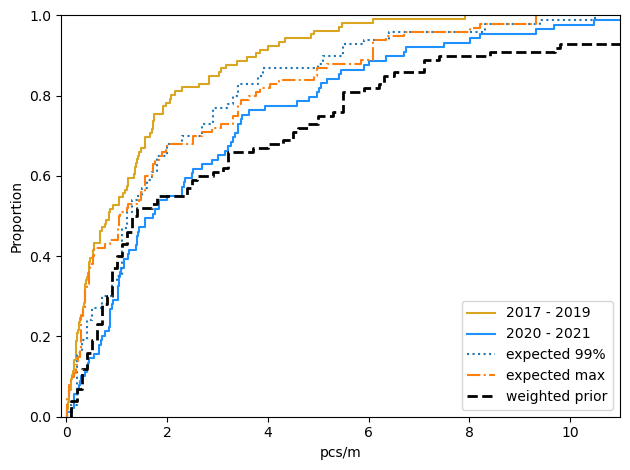
Forecast

Use case: Interpret forecasted values

All data

Minimum expected survey results 2025

Given the 99th percentile

• Average: 2.07

• HDI 95%: 0.1 - 6.4

• 90% Range: 0.2 - 6.4

Given the weighted prior

• Average: 3.49

• HDI 95%: 0.1 - 14.1

• 90% Range: 0.2 - 14.1

Given the observed max

• Average: 2.17

• HDI 95%: 0.02 - 8.21

• 90% Range: 0.13 - 9.33

Cumulative distribution of observed, sampling history and forecasts using to different priors.

Lakes

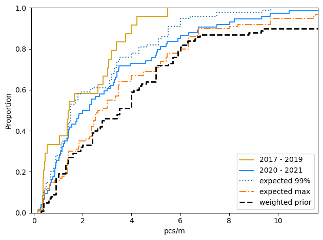
Minimum expected survey results 2025

Given the 99th percentile

• Average: 2.53

• HDI 95%: 0.3 - 6.4

• 90% Range: 0.4 - 6.02

Given the weighted prior

• Average: 5.95

• HDI 95%: 0.3 - 23.2

• 90% Range: 0.59 - 22.44

Given the observed max

• Average: 2.99

• HDI 95%: 0.16 - 9.68

• 90% Range: 0.37 - 10.47

Cumulative distribution of observed, sampling history and forecasts using to different priors.

Rivers

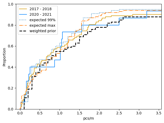
Minimum expected survey results 2025

Given the 99th percentile

• Average: 1.03

• HDI 95%: 0.1 - 3.9

• 90% Range: 0.1 - 2.57

Given the weighted prior

• Average: 1.43

• HDI 95%: 0.1 - 5.7

• 90% Range: 0.1 - 5.51

Given the observed max

• Average: 1.6

• HDI 95%: 0.02 - 6.08

• 90% Range: 0.06 - 4.91

Cumulative distribution of observed, sampling history and forecasts using to different priors.

Forecast methods

The applied method would best be classified as Empirical Bayes, in the sense that the prior is derived from the data (Bayesian Filtering and Smoothing or Empirical Bayes methods in classical and Bayesian inference). However, we share the concerns of Davidson-Pillon Bayesian methods for hackers about double counting and eliminate it the possibility as part of the formulation of the prior.

Model assumptions

1. Locations with similar land use attributes will have similar litter density rates

2. The data is a best estimate of what was present on the day of the survey

3. There are regional differences with respect to the density of specific objects

4. The locations surveyed are maintained by a public administration

The choice of land use features was a natural choice but was further explored in Near or Far.

Our parameter estimates are thus derived from the data and they remain testable and quantifiable according to Prior Probabilities, E T Jaynes. This makes our calculation very repetetive but also very well understood. It can be defined in a few lines of code for any set of survey results.

# standared libaries
import numpy as np
from scipy.stats import dirichlet, multinomial

# collect the data of interest
h = array of survey values

# count the number of times that each survey values exceed a value on the gird
counts = np.array([np.sum((h > x) & (h <= x + .1)) for x in grid_range])

# use the dirichlet dist to estimate p(Y >= x) for each x on the grid
# and sample from the estimation
adist = dirichlet(counts)
this_dist = adist.rvs(1-[0]

# draw samples from the conjugate
posterior_samples = multinomial.rvs(nsamples, p=this_dist)

Lakes and rivers sampled - all data

Lakes sampled

	samples	pcs/m
Bielersee	50	4.08
Brienzersee	5	3.96
Thunersee	43	1.21

Rivers sampled

	samples	pcs/m
Aare	61	1.27
Aarenidau-buren-kanal	3	1.26
Emme	9	0.60
Langeten	11	1.94
Schuss	2	1.04
Zulg	11	0.63

Municipal Results - all data

Use case: Where is the cleanest beach

The average pieces per meter and the combined land use classification for each city.

Lakes

	quantity	pcs/m	samples	orchards	vineyards	buildings	forest	undefined	public services	streets
city
Beatenberg	104	2.43	2	1	1	1	3	2	1	1
Biel/Bienne	3209	5.61	15	1	1	3	2	1	1	2
Brienz (BE)	696	4.49	3	1	1	2	2	3	1	2
Bönigen	277	3.18	2	1	1	3	2	2	1	2
Erlach	101	1.83	1	1	1	2	1	3	1	1
Gals	48	1.28	2	1	1	2	2	3	1	2
Ligerz	163	7.40	3	1	1	1	2	2	1	1
Lüscherz	202	0.75	5	1	1	1	3	1	1	1
Nidau	63	2.52	1	1	1	4	1	1	1	2
Spiez	838	0.79	26	1	1	2	2	3	1	1
Thun	276	1.40	3	1	1	5	1	1	1	2
Unterseen	1879	1.89	12	1	1	1	2	4	1	1
Vinelz	2033	3.77	23	1	1	2	1	3	1	2

Rivers

	quantity	pcs/m	samples	orchards	vineyards	buildings	forest	undefined	public services	streets
city
Belp	60	0.11	11	1	1	2	1	3	1	3
Bern	1892	1.02	32	1	1	3	1	2	1	3
Biel/Bienne	98	1.04	2	1	1	4	1	1	1	3
Brügg	36	1.02	1	1	1	3	2	2	1	3
Burgdorf	41	0.87	1	1	1	3	2	2	1	2
Kallnach	82	1.31	2	1	1	1	3	3	1	2
Köniz	757	2.86	12	1	1	4	1	1	1	4
Langenthal	301	1.94	11	1	1	3	1	2	1	2
Muri bei Bern	90	1.63	2	1	1	3	1	2	1	3
Port	118	1.38	2	1	1	3	2	2	1	3
Rubigen	57	3.20	1	1	1	1	1	4	1	2
Steffisburg	114	0.63	11	1	1	4	1	1	1	3
Utzenstorf	41	0.57	8	1	1	2	2	3	1	2
Walperswil	14	0.22	1	1	1	1	2	4	1	1