Land cover and land use#
The land cover and land use are used to determine the similarity of one survey location to another. In this way we can evaluate the probable minimum amount of trash at a given location based on the physical environment.
Land cover and land use provide information about the physical characteristics of a survey location. The land use and cover is measured by considering the proportion of land dedicated to specific purposes within a radius of 1’500 m of the survey location of interest. The specific puroposes are defined by the following map layers available at swissTLMRegio:
Landcover (TLM_BODENBEDECKUNG)
Streets (TLM_STRASSEN)
Hydrology (TLM_GEWAESSER)
Sports and recreation (TLM_FREIZEITAREAL)
Public services (TLM_NUTZUNGSAREAL)
Defining similar locations#
When comparing feature vectors in three-dimensional space, various distance metrics can be applied, each depending on the nature of the data and the type of comparison needed. Euclidean distance measures the straight-line distance between two points, making it suitable when the magnitude of differences in the same-scale features matters. Manhattan distance measures the sum of absolute differences across each dimension, which is useful when you prefer a more “axis-aligned” measure of difference, particularly when feature importance might vary along each axis. Cosine similarity, however, compares the orientation of the vectors in space, measuring how aligned they are regardless of magnitude. This is particularly relevant when the proportions between feature values are more important than their absolute values. In our analysis, cosine similarity was chosen because we are more interested in the relative proportions of the feature variables rather than their magnitudes.
Cosine similarity measures the cosine of the angle between two vectors in multi-dimensional space, focusing on the direction of the vectors rather than their length. The similarity ranges from -1 (perfectly opposite directions) to 1 (identical directions), with 0 indicating orthogonal or no similarity. The formula normalizes the vectors to unit length, comparing only the relative proportions between the dimensions. Cosine similarity is especially useful when the magnitude of the vectors varies significantly, but the pattern or trend of the features is important.
For example, imagine comparing two feature vectors:
\( x = [0.4, 0.5, 0.6] \)
\(y = [0.2, 0.25, 0.3] \)
Even though the absolute values of (y) are smaller than those of (x), the proportions between dimensions remain the same (i.e., \( 0.4/0.5 \approx 0.2/0.25\))). Cosine similarity will show that these two vectors are highly similar because their pattern or direction is nearly identical. By contrast, Euclidean distance would highlight the magnitude differences between the vectors, leading to a different measure of similarity.
Example: defining the land use for one location#
For each location the land use and land cover is calculated by first extracting the relevant features from the appropriate map layers within a radius of 1 500 m.
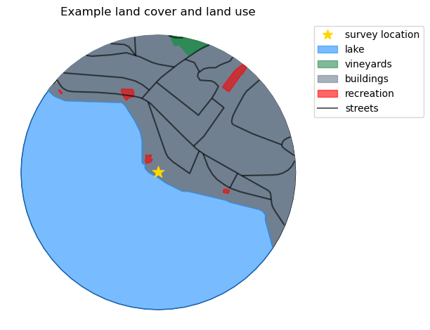
Land use profile#
The land use profile is the array of values between 0 and 1 that contains the proportion of the buffer zone occupied by the different land use and land cover attributes within the buffer zone of a survey location.
| location | vineyards | lake | buildings | recreation | streets | |
|---|---|---|---|---|---|---|
| 0 | quai-maria-belgia | 0.015907 | 1.284248 | 0.983656 | 0.015428 | 13894.013291 |
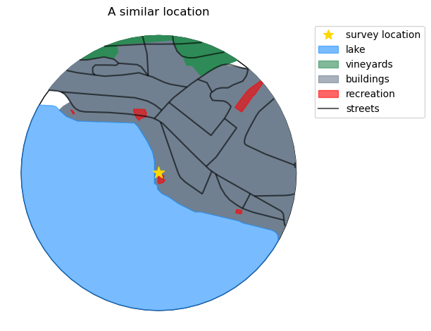
Finding similar locations#
The similarity of a location to other locations is determined by the cosine similarity, the manhattan distance or the euclidean distance between the land use profile of the location of interest and the land use profile of previously surveyed locations. The default method is cosine similarity, the default similarity threshold is 0.9.
| location | vineyards | lake | buildings | recreation | streets | |
|---|---|---|---|---|---|---|
| 0 | arabie | 0.069983 | 1.061684 | 0.914234 | 0.014763 | 17114.587103 |
Minimum Expected values#
The expected values are the minimum pcs/m we expect to find based on the survey results from similar locations.
In the case of locations that were previously sampled the minimum expected value is the conditional probability given the results from the location of interest and the results from similar locations.
For locations that have never been sampled#
The expected values or forecasts for a location that has never been sampled is the distribution of previous survey results from locations that meet the similarity threshold.
| pcs/m | |
|---|---|
| count | 50.000000 |
| mean | 1.161000 |
| std | 1.877075 |
| min | 0.000000 |
| 25% | 0.162500 |
| 50% | 0.450000 |
| 75% | 1.150000 |
| max | 8.180000 |
Using QGIS#
For this method we are using the land-cover layer from swissTLM regio
finished columns = slug, attribute , attribute_type, area, dry, scale
In QGIS:
create a buffer around each survey point
make sure that the survey location and feature_type is in the attributes of the new buffer layer
the survey locations are loaded as points from .csv file
reproject the points layer to the project CRS
use the new buffer layer as an overlay to the land-cover layer
use the overlay intersection tool
select the fields to keep from the buffer (slug and feature type)
select the fields to keep from the land-cover layer
run the function
this creates a temporary layer called intersection
get the surface area of all the land-cover and land-use features in each buffer of the temporary layer
use the field calculator for the attribute table of the layer
in the field calculator, make a new field and enter the formula
\$areafor this example the method is elipsoid bessel 1841 (epsg 7001)
this is set in the properties of the QGIS project
Export the layer as .csv
verify the land-use features per location
drop duplicate values: use location, feature and area to define duplicates
attention! different names for lake and reservoir
change Stausee to See
make a dry land feature
this is the surface area of the buffer that is not covered by water
substract the area of See from the area of the buffer
identify survey locations that have siginifcant water features but are not listed as lakes
Scale the land-use attributes of interest to the available dry-land
Author: hammerdirt-analyst

conda environment: cantonal_report

pandas    : 2.2.2
geopandas : 0.14.4
matplotlib: 3.8.4