1. Results 2015 - 2021

The MSFD protocol mlwguidance has been used on Lake Geneva since November 2015.

The data for this analysis is the results from beach-litter surveys conducted in Switzerland, on the shores of Lac Léman.

The data was collected according to the protocol described here https://www.plagespropres.ch/. In brief all visible data is collected along a beach within a measured distance from the waters edge. The width of the survey area depends on the terrain and the water level. The visible strand line or the nearest physical structure defines the width of a survey.

Surveys were conducted by the following organizations:

1. hammerdirt

2. Association pour le Sauvegarde du leman

3. Solid Waste Management Ecole Polytechnique Federal

4. Ecole International de Geneve

5. Precious plastic leman

This analysis is an open source document. The working notebook is available in the repository located here

Show code cell source Hide code cell source

%load_ext watermark

import os
import datetime as dt

# math packages:
import pandas as pd
import numpy as np
from scipy import stats
import datetime as dt 
from statsmodels.distributions.empirical_distribution import ECDF
from scipy.stats import percentileofscore

# charting:
import matplotlib as mpl
import matplotlib.pyplot as plt
import matplotlib.dates as mdates
from matplotlib import ticker
import seaborn as sns
import matplotlib.gridspec as gridspec

# documenting
# from IPython.display import display, HTML
from IPython.display import Markdown as md
from myst_nb import glue

glue("blank_caption", " ", display=False)

# all the data
survey_data = pd.read_csv("resources/data/u_pstk_iqaasl_all.csv")

survey_data["date"] = pd.to_datetime(survey_data["date"])
survey_data = survey_data[survey_data.code != "G216"].copy()

dfCodes = pd.read_csv("resources/data/u_codes.csv")
dfBeaches = pd.read_csv("resources/data/u_beaches.csv")

# map to code decriptions
dfCodes.set_index("code", inplace=True)

group_map = dfCodes["groupname"]

survey_data["groupname"] = survey_data.code.apply(lambda x: group_map.loc[x])

# leman and st sulpice data
coi = "Saint-Sulpice (VD)"

fd = survey_data.copy()

# the teams and the beaches they werre responsible for in each year
t_names = ["SWE", "PC", "EINT", "ASL", "SLR", "HD"]

teams_y1_4 = {
    "SWE":["tiger-duck-beach", "saint-sulpice", "rolle-plage", "plage-de-st-sulpice","parc-des-pierrettes"],
    "PC":["preverenges"],
    "EINT":["versoix",],
    "ASL":["baby-plage-geneva"],
    "SLR":["lacleman_vidy_santie", "lacleman_gland_lecoanets", "lacleman_gland_kubela"]
}

teams_y5_6 = {
    "SWE":["tiger-duck-beach", "saint-sulpice", "rolle-plage", "plage-de-st-sulpice","parc-des-pierrettes"],
    "PC":["preverenges", "maladaire", "vidy-ruines"],
    "EINT":["baby-plage-ii-geneve","rocky-plage"],
    "ASL":["baby-plage-geneva"],
    "SLR":[]
}

# hammerdirt was responsible for the surveys collected at the remaining locations
n_hd_y_1_4 = [*teams_y1_4[t_names[0]], *teams_y1_4[t_names[1]], *teams_y1_4[t_names[2]], *teams_y1_4[t_names[3]], *teams_y1_4[t_names[4]]]
n_hd_y_5_6 = [*teams_y5_6[t_names[0]], *teams_y5_6[t_names[1]], *teams_y5_6[t_names[2]], *teams_y5_6[t_names[3]], *teams_y5_6[t_names[4]]]

hd_y_1_4 = [x for x in fd.slug.unique() if x not in n_hd_y_1_4]
hd_y_5_5 = [x for x in fd.slug.unique() if x not in n_hd_y_5_6]

teams_y1_4.update({"HD":hd_y_1_4})
teams_y5_6.update({"HD":hd_y_5_5})

# this defines the css rules for the note-book table displays
header_row = {'selector': 'th:nth-child(1)', 'props': f'background-color: #FFF; text-align:right'}
even_rows = {"selector": 'tr:nth-child(even)', 'props': f'background-color: rgba(139, 69, 19, 0.08);'}
odd_rows = {'selector': 'tr:nth-child(odd)', 'props': 'background: #FFF;'}
table_font = {'selector': 'tr', 'props': 'font-size: 12px;'}
table_data = {'selector': 'td', 'props': 'padding: 6px;'}
table_caption = {'selector': 'caption', 'props': 'font-size: 14px; font-style: italic; caption-side: bottom; text-align: left; margin-top: 10px'}
table_css_styles = [even_rows, odd_rows, table_font, header_row, table_caption]

Show code cell source Hide code cell source

# set some parameters:
start_date = "2015-11-15"
end_date = "2021-11-14"

year_one = {"start_date":"2015-11-15", "end_date":"2016-11-14"}
year_two = {"start_date":"2016-11-15", "end_date":"2017-11-14"}
year_three = {"start_date":"2017-11-15", "end_date":"2018-11-14"}
year_four = {"start_date":"2018-11-15", "end_date":"2019-11-14"}
year_five = {"start_date":"2019-11-15", "end_date":"2020-11-14"}
year_six = {"start_date":"2020-11-15", "end_date":"2021-11-14"}

years = [year_one, year_two, year_three, year_four, year_five, year_six]
year_names = ["Year 1", "Year 2", "Year 3", "Year 4", "Year 5", "Year 6"]

fd["yx"] = ""
# make a column that has a value of year_names
def assign_a_survey_period(data, start_end, locs=[], year_name="Year 1"):
    """Slices the data by the start_end date and the locations in locs"""
    
    these_args = ((data["date"] >= start_end["start_date"])&(data["date"] <= start_end["end_date"])&(data["slug"].isin(locs)))
    data.loc[these_args, "yx"]= year_name   

for i,name in enumerate(year_names):
    assign_a_survey_period(fd, years[i], locs=fd.slug.unique(), year_name=name)    
    
for team in teams_y1_4:
    fd.loc[((fd.slug.isin(teams_y1_4[team]))&(fd["date"] < "2019-11-14")), "team"]= team

for team in teams_y5_6:
    fd.loc[((fd.slug.isin(teams_y5_6[team]))&(fd["date"] >= "2019-11-14")), "team"]= team

fd = fd[fd.yx.isin(year_names)].copy()

samples per team per year

Show code cell source Hide code cell source

a = fd.groupby(["yx", "team"], as_index=False).agg({"loc_date":"nunique", "quantity":"sum"})
asamps = a.pivot(columns="team", index="yx", values="loc_date").fillna(0).astype("int")
asamps.loc[:, "Total"] = asamps.sum(axis=1)
caption = "Table 1, number of samples per team per year"
asamps.to_csv("output/csvs/table_1.csv", index=False)
asamps.index.name = None
table_1 = asamps.style.set_caption(caption).set_table_styles(table_css_styles)

table_1

Table 1, number of samples per team per year

team	ASL	EINT	HD	PC	SLR	SWE	Total
Year 1	0	0	80	0	0	2	82
Year 2	0	1	28	0	17	2	48
Year 3	0	0	6	2	15	2	25
Year 4	0	0	0	0	0	2	2
Year 5	5	2	33	16	0	4	60
Year 6	6	1	24	16	0	3	50

pieces per team per year

Show code cell source Hide code cell source

aqty = a.pivot(columns="team", index="yx", values="quantity").fillna(0).astype("int")
aqty.loc[:, "Total"] =  aqty.sum(axis=1)

caption = "Table 2, pieces per team per year"
aqty.to_csv("output/csvs/table_2.csv", index=False)
aqty.index.name = None
table_2 = aqty.style.set_caption(caption).set_table_styles(table_css_styles)

table_2

Table 2, pieces per team per year

team	ASL	EINT	HD	PC	SLR	SWE	Total
Year 1	0	0	28007	0	0	2721	30728
Year 2	0	1490	10188	0	2526	1006	15210
Year 3	0	0	2164	203	1591	1534	5492
Year 4	0	0	0	0	0	306	306
Year 5	2719	167	9582	4701	0	1536	18705
Year 6	556	20	6130	2072	0	971	9749

median pieces per sample per team

Show code cell source Hide code cell source

a["qs"] = a["quantity"]/a["loc_date"]
aqs = a.groupby("team", as_index=False).qs.median()

caption = "Table 3, median pieces per sample per team"
aqs.to_csv("output/csvs/table_3.csv", index=False)
aqs.index.name = None
aqs=aqs.T
aqs.rename(columns={x:aqs.loc["team"].values[x] for x in aqs.columns}, inplace=True)
aqs.drop('team', inplace=True)
# aqs.set_index("team", drop=True, inplace=True)
aqs.index.name = None
table_3 = aqs.style.format(precision=2).set_caption(caption).set_table_styles(table_css_styles)

table_3

Table 3, median pieces per sample per team

	ASL	EINT	HD	PC	SLR	SWE
qs	318.23	83.50	350.09	129.50	127.33	443.50

1.1. Variation in trash over time

The median survey value at the end of year 6 is less than all previous years, this corresponds to the results from the national survey that was terminated in May 2021. However, the 25th percentile from year one is less than the median from year six. This suggests that at least 50% of the samples from year six would have been below the 25th percentile of the first year. Given these results it is possible that there were reductions at specific locations, because 50% of the samples in year six fall below the IQR of year one.

1.1.1. Year over year summary statistics

Show code cell source Hide code cell source

a_l = fd.groupby(["yx", "loc_date", "slug", "team"], as_index=False).agg({"pcs/m":"sum", "quantity":"sum", })
a_l_summary = a_l.groupby("yx").agg({"loc_date":"nunique", "pcs/m":["median", "mean", "var"], "slug":"nunique", "quantity":"sum"})
a_l_summary.columns = ["samples", "median", "mean","var", "locations", "pieces"]
a_l_summary["dispersion"] = a_l_summary["var"]/a_l_summary["mean"]
# a_l_summary.round(2)

aqs = a_l_summary.round(2)
caption = "Table 4, year over year summary statistics"
aqs.to_csv("output/csvs/table_4.csv", index=False)
aqs.index.name = None
# aqs.set_index("team", drop=True, inplace=True)
# aqs.index.name = None
table_4 = aqs.style.format(precision=2).set_caption(caption).set_table_styles(table_css_styles)

table_4

Table 4, year over year summary statistics

	samples	median	mean	var	locations	pieces	dispersion
Year 1	82	4.86	8.77	98.63	18	30728.00	11.24
Year 2	48	6.36	8.49	62.97	19	15210.00	7.42
Year 3	25	4.53	8.88	249.97	11	5492.00	28.14
Year 4	2	7.53	7.53	9.86	2	306.00	1.31
Year 5	60	5.57	9.39	145.54	22	18705.00	15.50
Year 6	50	3.87	7.15	101.88	22	9749.00	14.24

The dispersion (variance/mean) is greater than one for all years, prohibiting the use of a Poisson distribution but supporting the EUs decision to model outliers based on the Negative Binomial distributioneubaseleines.

Show code cell source Hide code cell source

fig, ax = plt.subplots(figsize=(8,6))
data = fd[fd.yx.isin(["Year 1", "Year 6"])].groupby(["loc_date", "yx"], as_index=False).agg({"pcs/m":"sum"})
iq = fd[fd.yx == "Year 1"].groupby(["loc_date"])["pcs/m"].sum().to_numpy()

twenty_five, seventy_five = np.round(np.percentile(iq, 25), 2), np.round(np.percentile(iq, 75), 2)


data.to_csv("output/csvs/figure_1.csv", index=False)

sns.histplot(data=data, x="pcs/m", hue="yx", ax=ax, zorder=2, label="yx", multiple="stack")

ax.vlines([twenty_five, seventy_five], ymin=0, ymax=30, linestyle="dashed", color="dodgerblue", zorder=3, linewidths=2)
ax.fill_between([np.percentile(iq, 25), np.percentile(iq, 75)], y1=0, y2=30, color="dodgerblue", alpha=0.3, zorder=0, label=f"50% IQR year one: [{twenty_five}, {seventy_five}]")
h,l = ax.get_legend_handles_labels()
hs = h[0]
nl = [l[0], "Year 1", "Year 6"]
plt.legend(h,nl, frameon=False)

ax.set_ylabel("Number of samples", fontsize=14)
ax.set_xlabel("Pieces per meter", fontsize=14)
plt.tight_layout()
glue("figure-1-swe", fig, display=False)
plt.close()

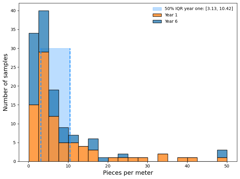
Fig. 1.1

figure 1.1: Survey results from year one compared to year two.

Show code cell source Hide code cell source

fig, ax = plt.subplots(figsize=(8,6))
data = fd.groupby(["loc_date"], as_index=False).agg({"pcs/m":"sum"})
data.to_csv("output/csvs/figure_2.csv", index=False)
sns.histplot(data=data, x="pcs/m",ax=ax, zorder=2)

ax.set_ylabel("Number of samples", fontsize=14)
ax.set_xlabel("Pieces per meter", fontsize=14)

plt.tight_layout()

glue("figure-2-swe", fig, display=False)
plt.close()

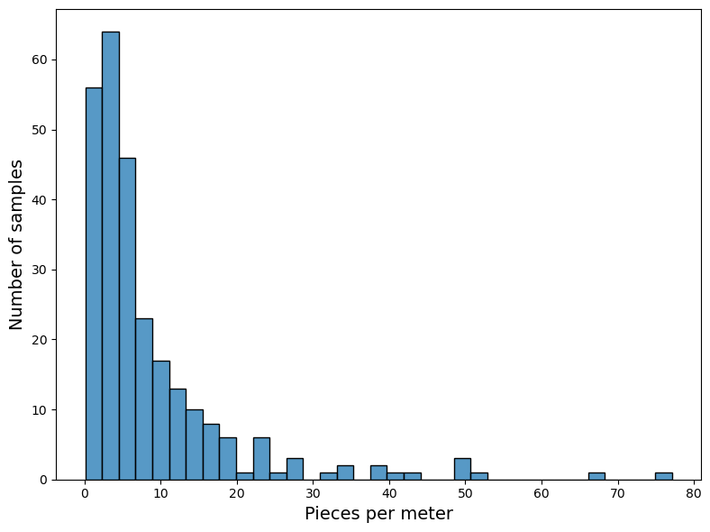
Fig. 1.2

figure 1.2: Distribution of surveys 2015 - 2021

Show code cell source Hide code cell source

fig, ax = plt.subplots(figsize=(8,6))
a_locdate = fd.groupby(["loc_date","date", "slug", "team"], as_index=False).agg({"pcs/m":"sum", "quantity":"sum", })
a_locdate["date"]=pd.to_datetime(a_locdate["date"])

a_locdate.to_csv("output/csvs/figure_3.csv", index=False)

ylimit=60
sns.scatterplot(data=a_locdate, x="date", y="pcs/m", s=50, hue="team")
ax.set_xlabel("")
days = mdates.DayLocator(interval=7)

ax.tick_params(axis="x", which="major", pad=15)

ax.set_ylim(-.5,60)
ax.set_ylabel("Pieces per meter", fontsize=14)
ax.legend(loc="upper right", fancybox=False, facecolor="white", edgecolor='0.0', framealpha=1)
ax.legend().get_frame().set_linewidth(0)
glue("figure-3-swe", fig, display=False)
plt.close()

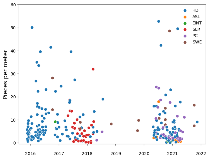
Fig. 1.3

figure 1.3: Survey results since 2015.

1.1.2. Survey total summary

Table 5, Summary statistics of the daily total in pcs or trash per meter. All objects included

	count	mean	std	min	25%	50%	75%	max
pcs/m	267.00	8.56	10.74	0.09	2.59	4.94	9.72	77.10

Below The year over year survey results for Lac Léman. There are surveys in each year since 2015

Show code cell source Hide code cell source

a_locdate = fd.groupby(["yx", "loc_date","date", "slug", "team"], as_index=False).agg({"pcs/m":"sum", "quantity":"sum", })
a_locdate["date"]=pd.to_datetime(a_locdate["date"])

a_locdate.to_csv("output/csvs/figure_4.csv", index=False)

PROPS = {
    'boxprops':{'facecolor':'none'},   
}

fig, ax = plt.subplots(figsize=(8,6))

sns.boxplot(data=a_locdate, x="yx", y="pcs/m", showfliers=False, ax=ax, **PROPS, zorder=2, order=year_names)
sns.stripplot(data=a_locdate, x="yx", y="pcs/m", ax=ax, size=8, alpha=.6,hue="team", jitter=.3, zorder=0, order=year_names)
ylimit = np.quantile(a_locdate["pcs/m"].values, .99)
ax.set_ylim(0, ylimit)
ax.set_ylabel("pcs/m", fontsize=14)
ax.set_xlabel("")
ax.legend(loc="upper right", fancybox=False, facecolor="white", edgecolor='0.0', framealpha=1)
ax.legend().get_frame().set_linewidth(0)

glue("figure-4-swe", fig, display=False)
plt.close()

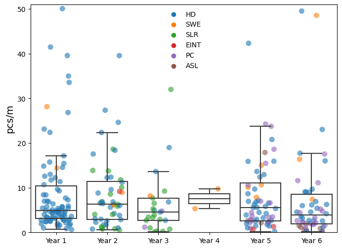
Fig. 1.4

figure 1.4: The 90% interval of the survey results year over year.

Show code cell source Hide code cell source

axis_limits = ylimit
statement = f"Values greater than {np.round(ylimit, 2)} pcs/m not shown, the 99th percentile."
md(statement)

Values greater than 50.97 pcs/m not shown, the 99th percentile.

1.1.3. Year over year cumulative distribution

Considering sample years with more than two observations. The highest median was in year 2 and the highest mean was recorded in years 2 and 5 but the maximum value was recorded in year 3 by SWE students at tiger-duck-beach. The dispersion is lowest in year two. The third year has the lowest number of samples and locations but the highest dispersion. Three locations are responsible for 68% of all samples in year three. The median survey value of these three locations ranges from 0.29 to 6.5, the maximum survey value in year three was 77pcs/m. Differences of this magnitude are regular occurrences, the high variance of beach litter surveys was noted when the EU published guidelines on determining baseline values and thresholds. eubaselines

Show code cell source Hide code cell source

ecdfs = [ECDF(a_locdate[a_locdate.yx == x]["pcs/m"].values) for x in year_names]
sns.set_style("whitegrid")


fig, ax = plt.subplots(figsize=(5,5))

ax.set_xlim(0, ylimit)


for i, name in enumerate(year_names):
    if i == 0:
        somdata=ecdfs[0].x
        median = np.quantile(a_locdate[a_locdate.yx == name]["pcs/m"].values, .5)
        lower25 = np.quantile(a_locdate[a_locdate.yx == name]["pcs/m"].values, .25)
        upper25 = np.quantile(a_locdate[a_locdate.yx == name]["pcs/m"].values, .75)
        ax.vlines([lower25, upper25], ymin=0, ymax=1, linestyle="dashed", color="dodgerblue", zorder=1, linewidths=1)
        ax.fill_between([lower25, upper25], y1=0, y2=1, color="dodgerblue", alpha=0.3, zorder=0, label="Year 1 IQR")
        ax.vlines(median, ymin=0, ymax=1, color="red", linestyle="dashdot", linewidths=2, alpha=1, zorder=3)
        
        
    if i != 3:
        sns.lineplot(x=ecdfs[i].x, y=ecdfs[i].y, ax=ax, label=name, zorder=2)
        
    else:
        pass
handles, labels = ax.get_legend_handles_labels()
ax.set_xlabel("pcs/m", fontsize=14)
ax.set_ylabel("Cumulative probability", fontsize=14)

n_handles = [handles[-1], *handles[:-1]]
n_labels = [labels[-1], *labels[:-1]]    
plt.legend(n_handles, n_labels, bbox_to_anchor=(1,1), fancybox=False, facecolor="white", edgecolor='0.0', framealpha=1)
ax.legend().get_frame().set_linewidth(0)
plt.title(f"Year one IQR = [{round(lower25, 2)}, {round(upper25, 2)}]", loc='left')
plt.tight_layout()
glue("figure-5-swe", fig, display=False)
plt.close()

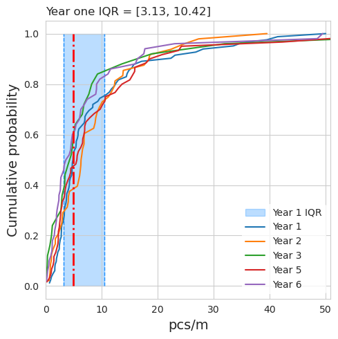
Fig. 1.5

figure 1.5: Cumulative distribution year over year

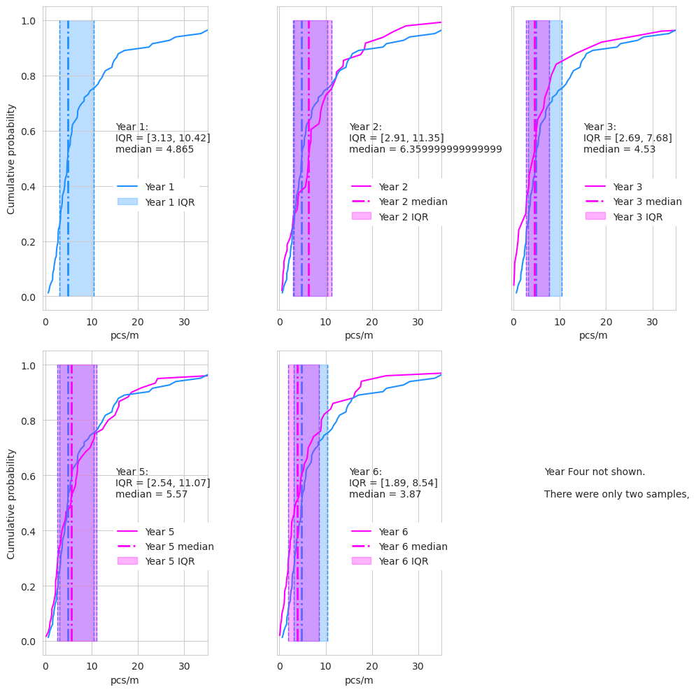
Fig. 1.6

figure 1.6: Cumulative distribution year over year

1.1.4. Comparison between the survey groups

The innerquartile range from y-one accounts for 50% of the survey results from SLR and 59% of the results from PC. The 25^th percentile is much lower in both cases (Fig. 5). The groups also represent regional clusters. The year one surveys were primarily from the Haut Lac, SLR surveys are primarily in the Grand Lac and PC surveys are between the Grand Lac and the Haut Lac. The variance between years and groups has a part that can be attributed to location.

Show code cell source Hide code cell source

ecdfs = [ECDF(a_locdate[a_locdate.team == x]["pcs/m"].values) for x in ["HD", "SLR", "PC"]]
sns.set_style("whitegrid")
colors = ["dodgerblue", "magenta", "saddlebrown"]


fig, ax = plt.subplots(figsize=(5,6))

ax.set_xlim(0, 35)

iqrs_by_group = {}

for i, name in enumerate(["HD", "SLR", "PC"]):
    somdata=ecdfs[i].x
    ecdfs.append(somdata)
    median = np.quantile(somdata, .5)
    lower25 = np.quantile(somdata, .25)
    upper25 = np.quantile(somdata, .75)
    iqrs_by_group.update({name:[lower25, median, upper25]})    
    
    ax.fill_between([lower25, upper25], y1=0, y2=1, color=colors[i], alpha=0.3, zorder=0, label=f"IQR {name}")
    sns.lineplot(x=ecdfs[i].x, y=ecdfs[i].y, ax=ax, label=name, zorder=1, color=colors[i])
        
combined = ECDF([*ecdfs[0].x, *ecdfs[1].x, *ecdfs[2].x])

sns.lineplot(x=combined.x, y=combined.y, ax=ax, label="Combined surveys", zorder=2, linestyle="dashed", color="black")

handles, labels = ax.get_legend_handles_labels()
ax.set_xlabel("pcs/m", fontsize=14)
ax.set_ylabel("Cumulative probability", fontsize=14)

n_handles = [*handles[-4:], *handles[:-4]] # handles
n_labels =  [*labels[-4:], *labels[:-4]] # labels
ax.legend(n_handles, n_labels, bbox_to_anchor=(1,1), fancybox=False, facecolor="white", edgecolor='0.0', framealpha=1)
ax.legend().get_frame().set_linewidth(0)
glue("figure-6-swe", fig, display=False)
plt.close()

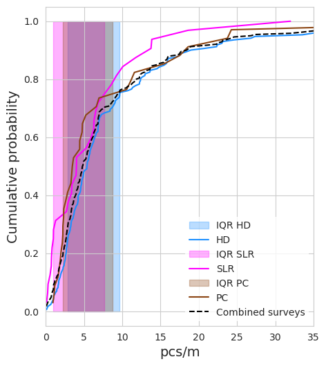
Fig. 1.7

figure 1.7: Cumulative distribution by survey group

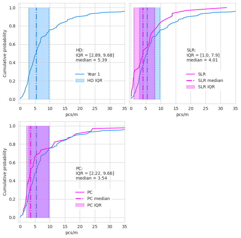
Fig. 1.8

figure 1.8: Detail of the cumulative distribution of the different survey groups compared to each other.

The number of locations below the 25th and above the 75th percentile

Consider the results from year one as a base year and recall that HD was responsible for 80 of the 82 surveys. SLR has 12 samples below the IQR from year one and 5 above the IQR. Aproximately 46% of SLR surveys fall within the IQR of year one. PC had 14 below the IQR and seven above or 38% of all PC surveys fall within the IQR of year one.

1.2. Composition over time

Year over percent of total of the top ten codes on Lake Geneva

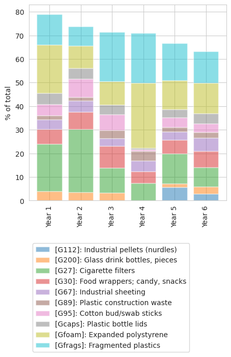
Fig. 1.9

figure 1.9: Year over year percent of total of the top ten objects on Lake Geneva

Table of values year over year percent of total of the top ten codes on Lake Geneva

Show code cell source Hide code cell source

caption = "Table 6, Summary statistics of the daily total in pcs or trash per meter. All objects included"
p_total_yoy.to_csv("output/csvs/table_6.csv", index=False)
p_total_yoy.index.name = None
p_total_yoy = p_total_yoy[p_total_yoy.columns[::-1]]

caption = "Table 6: Year over year percent of total of the top ten objects Lake Geneva."
table_6 = p_total_yoy.style.format(precision=2).set_caption(caption).set_table_styles(table_css_styles)

table_6

Table 6: Year over year percent of total of the top ten objects Lake Geneva.

code	Gfrags	Gfoam	Gcaps	G95	G89	G67	G30	G27	G200	G112
Year 1	13.00	20.50	4.60	4.90	1.70	4.10	6.20	20.00	4.00	0.00
Year 2	8.20	9.50	4.50	7.70	1.60	4.70	7.40	26.70	3.50	0.00
Year 3	21.00	9.80	4.30	6.60	3.50	3.20	9.30	10.50	3.30	0.00
Year 4	21.20	27.50	0.70	0.70	3.90	4.60	4.90	7.50	0.00	0.00
Year 5	15.60	12.40	3.40	4.00	2.00	3.50	5.70	12.80	1.40	5.80
Year 6	13.30	13.00	4.20	3.70	2.50	5.60	6.90	8.00	3.00	3.00

Show code cell source Hide code cell source

p_total_yoy = ten_yoy[ten_yoy.code.isin(lake_top_ten)].pivot(index="code", columns="yx", values="quantity")
p_yoy = p_total_yoy.sort_values(by="Year 1", ascending=False)
p_yoy.loc["total"] = p_yoy.sum(axis=0)


aqs = p_yoy

caption = "Table 7, Summary statistics of the daily total in pcs or trash per meter. All objects included"
# aqs.to_csv("output/csvs/table_7.csv", index=False)
aqs.index.name = None
# aqs.astype("int")

caption = "Table 7, Year over year quantity of the top ten objects."
table_7 = aqs.style.format(precision=0).set_caption(caption).set_table_styles(table_css_styles)

table_7

Table 7, Year over year quantity of the top ten objects.

yx	Year 1	Year 2	Year 3	Year 4	Year 5	Year 6
Gfoam	6298	1442	536	84	2318	1271
G27	6152	4068	579	23	2392	777
Gfrags	3985	1243	1151	65	2923	1297
G30	1913	1119	509	15	1069	668
G95	1498	1174	362	2	754	358
Gcaps	1421	686	236	2	640	410
G67	1246	713	174	14	658	542
G200	1234	533	183	0	261	293
G89	524	247	190	12	366	248
G112	0	0	0	0	1091	296
total	24271	11225	3920	217	12472	6160

1.2.1. Composition over time Saint Sulpice

The top ten from all samples in Saint-Sulpice year over year.

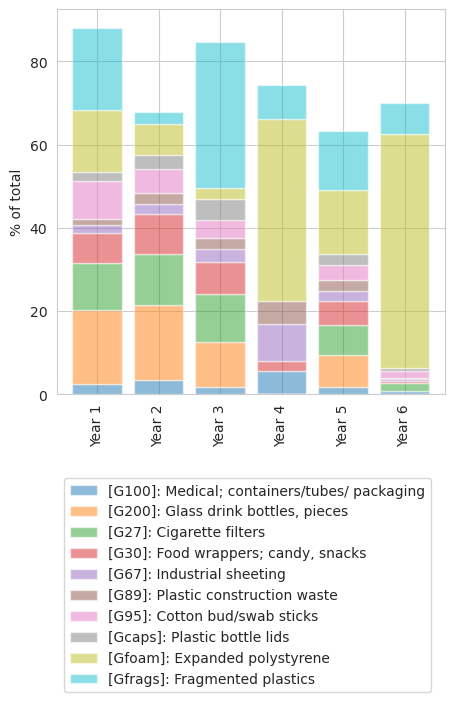
Fig. 1.10

figure 1.10: Year over percent of total of the top ten Saint Sulpice

Table of values values percent of total of the top ten Saint Sulpice

Table 8: Percent total year over year Saint Sulpice

code	G100	G200	G27	G30	G67	G89	G95	Gcaps	Gfoam	Gfrags
Year 1	2.50	17.80	11.20	7.40	1.70	1.50	9.20	2.20	14.90	19.70
Year 2	3.50	18.10	12.20	9.50	2.40	2.60	5.80	3.40	7.60	2.70
Year 3	1.90	10.60	11.60	7.80	3.00	2.60	4.40	5.10	2.50	35.10
Year 4	5.60	0.00	0.00	2.50	8.80	5.60	0.00	0.00	43.80	8.10
Year 5	1.80	7.60	7.20	5.90	2.30	2.80	3.60	2.50	15.50	14.20
Year 6	0.80	0.00	1.90	0.60	0.40	0.30	1.60	0.80	56.10	7.50

1.3. Site specific results

As mentioned previously the SWE group is the only group that has surveys in each year in the same municipality. Of the beaches surveyed by SWE, two are separated by a short walk through a residential neighborhood. The year over year results from Plage de St-Sulpice (PS) and Parc des Pierrettes (PP) were compared to the base year median set in sampling period one. Both beaches had results greater than the lake median in each year but the pcs/m at each site declined year over year with respect to the first sample. This corresponds with the observations in the previous section reference y-one and y-six. If there is a general trend it appears that these two locations are following it.

Table 9, The difference in survey results from the base year (diff-by) and the first sample (diff-y1) at Plage de St Sulpice and Parc des Pierettes.

	yx	loc_date	slug	pcs/m	quantity	dif-by	dif-y1
0	Year 1	('parc-des-pierrettes', '2016-10-13')	parc-des-pierrettes	14.39	693.00	9.53	0.00
1	Year 1	('plage-de-st-sulpice', '2016-10-13')	plage-de-st-sulpice	28.13	2028.00	23.27	0.00
2	Year 2	('parc-des-pierrettes', '2017-10-05')	parc-des-pierrettes	6.15	258.00	1.29	-8.24
3	Year 2	('plage-de-st-sulpice', '2017-10-05')	plage-de-st-sulpice	8.92	748.00	4.06	-19.21
4	Year 4	('parc-des-pierrettes', '2019-10-10')	parc-des-pierrettes	5.31	160.00	0.45	-9.08
5	Year 5	('parc-des-pierrettes', '2020-10-01')	parc-des-pierrettes	10.08	464.00	5.22	-4.31
6	Year 5	('plage-de-st-sulpice', '2020-10-01')	plage-de-st-sulpice	7.85	326.00	2.99	-20.28
7	Year 6	('plage-de-st-sulpice', '2021-10-07')	plage-de-st-sulpice	7.40	0.00	2.54	-20.73

Upon collection and sorting, the quantity of each material type was input into the database based on the MLW code classification. Figure x and y (quantities presented in Appendix – Table 5 & 6) show the segmented data for the litter collected at Plage de St-Sulpice (PS) and Parc des Pierrettes (PP) beaches.

Scrutinizing the data further, it can be seen that the majority of the litter is composed of plastics that accounts for approximately 69 and 88% for both PS and PP, respectively.

Table 10, Material composition of the objects identified at the locations of interest

slug	parc-des-pierrettes	plage-de-st-sulpice
Chemicals	0.06	0.00
Cloth	0.95	0.42
Glass	7.30	24.89
Metal	1.59	3.06
Paper	1.21	0.52
Plastic	88.19	69.76
Rubber	0.38	0.93
Unidentified	0.00	0.00
Wood	0.32	0.42

Via categorising the AL in accordance to the MLW, and comparing the total surveyed data, it is shown that even with the appearance of the same physical material, in this case predominantly composed of polymeric material, the source it originates from is different along with the quantity. Most probably, the reason for the difference could be the flow in the lake. It takes approximately 10 years for the volume of water to pass through the lake (residence time), and at the same time seasonal fluctuation and the direction of the beach can affect where and by how much the waste accumulates. For instance, the PS beach is somewhat sheltered from the directional flow of water, and thus there is a higher potential of debris accumulating there over time. PP is mostly parallel to the flow and thus, it attracts a different type of waste. Thus, a quantitative assessment as such helps gain insight as to how ‘healthy’ the shoreline is when used for recreational activities based on the location relative to the flow.

Show code cell source Hide code cell source

code_summary = fdsp[fdsp.yx.isin(["Year 1", "Year 2", "Year 5"])].groupby(["slug", "code", "groupname"], as_index=False).quantity.sum()
for code in code_summary.code.unique():
    code_summary.loc[code_summary.code == code, "description"] = code_d.loc[code]
    code_summary.loc[code_summary.code == code, "material"] =  mat_d.loc[code]

c_sum = []
for each_beach in boi:
    tten = code_summary[code_summary.slug ==each_beach].sort_values(by="quantity", ascending=False)[:10]
    mat = code_summary[code_summary.slug ==each_beach][["material", "quantity"]].groupby("material", as_index=False).quantity.sum().sort_values(by="quantity", ascending=False)
    groups = code_summary[code_summary.slug ==each_beach][["groupname", "quantity"]].groupby("groupname", as_index=False).quantity.sum().sort_values(by="quantity", ascending=False)
    
    c_sum.append([tten, mat, groups])

1.3.1. Plage de Saint Sulpice:

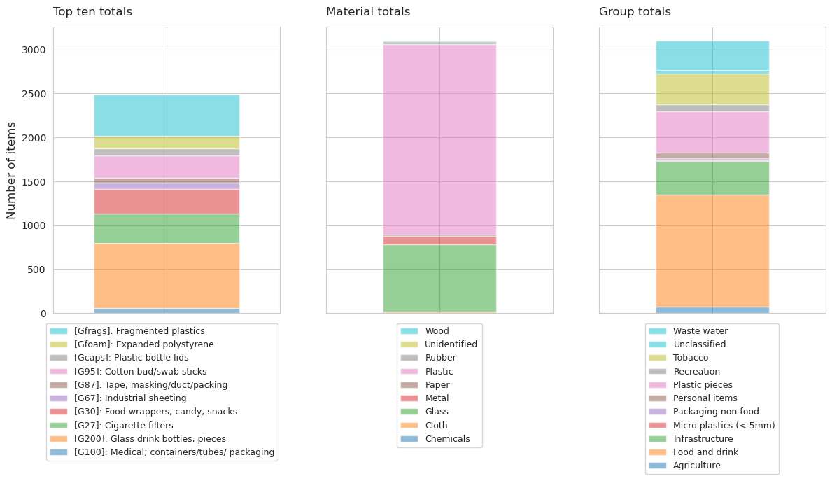
Fig. 1.11

figure 1.11: The quantity of the top-ten items and their material composition as well as use or size classification

Top ten totals plage-de-st-sulpice

	description	quantity
274	Glass drink bottles, pieces	737.00
351	Fragmented plastics	475.00
289	Cigarette filters	341.00
293	Food wrappers; candy, snacks	279.00
343	Cotton bud/swab sticks	252.00
350	Expanded polystyrene	142.00
349	Plastic bottle lids	82.00
325	Industrial sheeting	65.00
334	Tape, masking/duct/packing	59.00
178	Medical; containers/tubes/ packaging	57.00

1.3.2. Parc des Pierettes

Show code cell source Hide code cell source

tdata = c_sum[1][0].pivot(columns="code", index="slug", values="quantity")

matdata = c_sum[1][1].copy()
matdata["slug"] = "slug"
matdata = matdata.sort_values(by='quantity', ascending=False).pivot(columns='material', index="slug", values='quantity')

gdata = c_sum[1][2]
gdata["slug"] = "slug"
gdata = gdata.sort_values(by='quantity', ascending=False).pivot(columns='groupname', index="slug", values='quantity')
    
fig, ax = plt.subplots(1,3, figsize=(12,7), sharey=True)

tdata.plot.bar(stacked=True, colormap='tab10', alpha=0.5, ax=ax[0], width=.9)

ax[0].tick_params(axis='x',  which='both',  bottom=False, labelbottom=False, labelsize=0)
h, ls = ax[0].get_legend_handles_labels()
new_labels = [f'[{x}]: {code_d[x]}' for x in ls]
ax[0].legend(h[::-1], new_labels[::-1], bbox_to_anchor=(0, -.02), loc='upper left', ncol=1,fontsize=9)
ax[0].set_title("Top ten totals", pad=12, fontsize=12, loc='left')
ax[0].set_ylabel("Number of items", fontsize=12)
ax[0].set_xlabel("")

matdata.plot.bar(stacked=True, colormap='tab10', alpha=0.5, ax=ax[1])
h, ls = ax[1].get_legend_handles_labels()
ax[1].tick_params(axis='x',  which='both',  bottom=False, labelbottom=False, labelsize=0)
ax[1].legend(h[::-1], ls[::-1], bbox_to_anchor=(0.5, -.02), loc='upper center', ncol=1,fontsize=9)
ax[1].set_title("Material totals", pad=12, fontsize=12, loc='left')
ax[1].set_ylabel("Ylabel", fontsize=14)
ax[1].set_xlabel("")

gdata.plot.bar(stacked=True, colormap='tab10', alpha=0.5, ax=ax[2])
h, ls = ax[2].get_legend_handles_labels()
ls = [x.capitalize() for x in ls]
ax[2].tick_params(axis='x',  which='both',  bottom=False, labelbottom=False, labelsize=0)
ax[2].legend(h[::-1], ls[::-1], bbox_to_anchor=(0.5, -.02), loc='upper center', ncol=1,fontsize=9)
ax[2].set_title("Group totals", pad=12, fontsize=12, loc='left')
ax[2].set_ylabel("Ylabel", fontsize=14)
ax[2].set_xlabel("")

plt.tight_layout()

glue("figure-10-swe", fig, display=False)
plt.close()

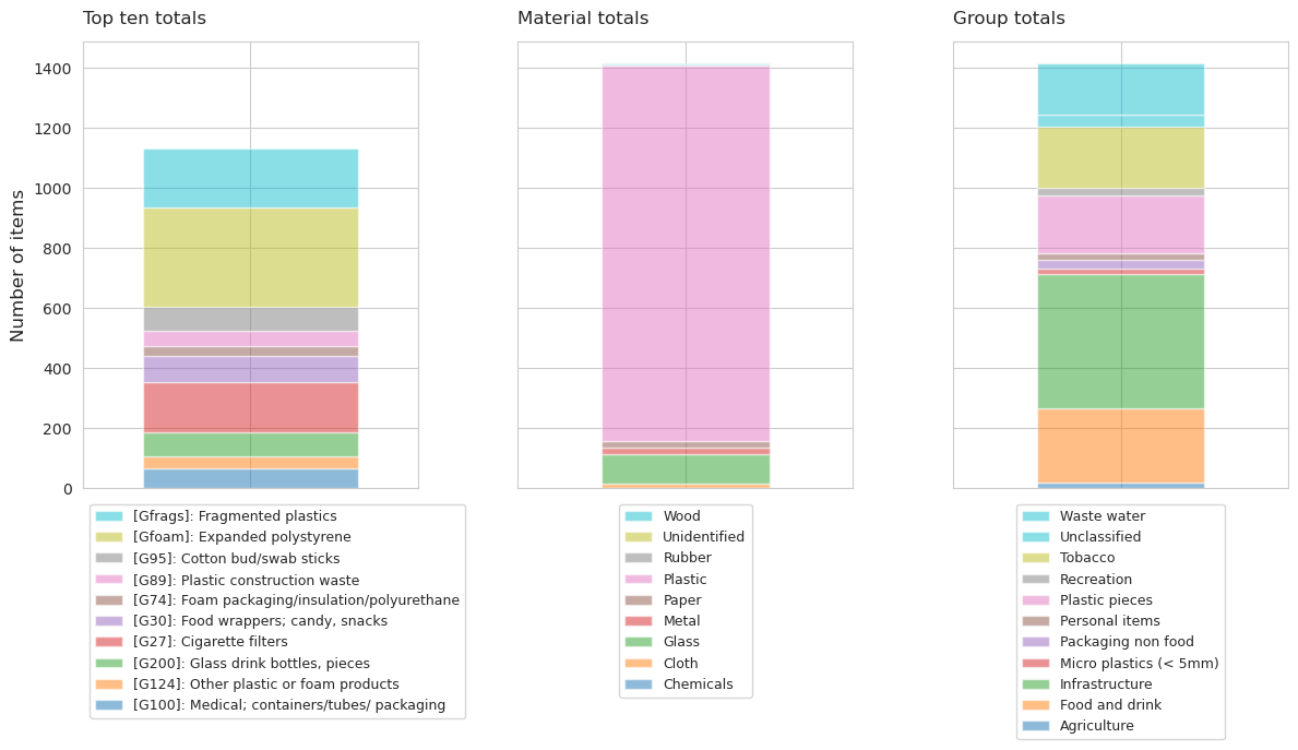
Fig. 1.12

figure 1.12: The quantity of the top-ten items and their material composition as well as use or size classification

Top ten totals parc-des-pierrettes

	description	quantity
174	Expanded polystyrene	333.00
175	Fragmented plastics	195.00
113	Cigarette filters	169.00
117	Food wrappers; candy, snacks	86.00
167	Cotton bud/swab sticks	80.00
98	Glass drink bottles, pieces	80.00
2	Medical; containers/tubes/ packaging	66.00
160	Plastic construction waste	49.00
25	Other plastic or foam products	39.00
155	Foam packaging/insulation/polyurethane	34.00

1.3.2.1. Distribution of top-ten

At PS all the most common items had lower survey values when compared to year one, at PP it was 6 out of 10. In both cases cigarette ends and broken glass are both less in the last survey year. This also corresponds to the general trend observed in the national report. St Sulpice is moderately dense and would be considered urban under most circumstances.

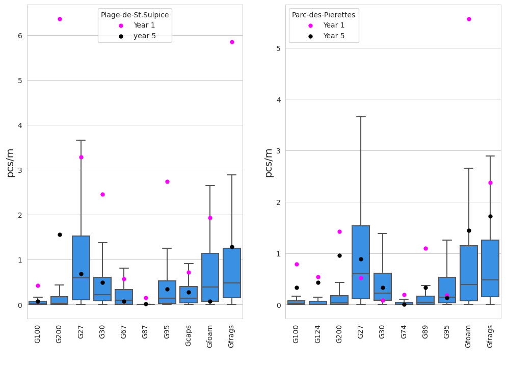
Fig. 1.13

figure 1.13: At PS all the most common items had lower survey values when compared to year one, at PP it was 6 out of 10. In both cases cigarette ends and broken glass are both less in the last survey year. This also corresponds to the general trend observed in the national report. St Sulpice is moderately dense and would be considered urban under most circumstances.

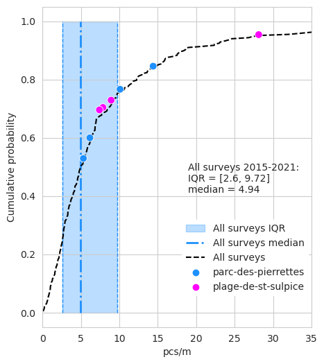
Fig. 1.14

figure 1.14: At PS all the most common items had lower survey values when compared to year one, at PP it was 6 out of 10. In both cases cigarette ends and broken glass are both less in the last survey year. This also corresponds to the general trend observed in the national report. St Sulpice is moderately dense and would be considered urban under most circumstances.

Top ten totals parc-des-pierrettes

	slug	pcs/m	p
0	parc-des-pierrettes	14.39	0.85
1	parc-des-pierrettes	6.15	0.60
2	parc-des-pierrettes	5.31	0.53
3	parc-des-pierrettes	10.08	0.77
4	plage-de-st-sulpice	28.13	0.95
5	plage-de-st-sulpice	8.92	0.73
6	plage-de-st-sulpice	7.85	0.70
7	plage-de-st-sulpice	7.40	0.70

This script updated 09/10/2023 in Biel, CH

❤️ what you do everyday: analyst at hammerdirt

Git repo: https://github.com/hammerdirt-analyst/solid-waste-team.git

Git branch: main

pandas    : 2.0.2
numpy     : 1.24.3
matplotlib: 3.7.1
seaborn   : 0.12.2
scipy     : 1.10.1