3. Testing 2023 predictions

3.1. The solid waste experience

This is the seventh year that the Solid Waste Team from the EPFL collect beach litter samples. In the maritime environment people have been measuring beach litter for decades. There is a standard protocol (Guidance on Monitoring Marine Litter in European Seas) for the EU area and threshold values for good environmental standing (Beach litter thresholds).

In Switzerland we started monitoring shoreline trash in 2015, it was not obvious to most observers (except for Prof Ludwig) why this might be of interest. However, by 2016 the EU realized that monitoring trash flows in rivers and lakes (monitoring trash in rivers) might be a good way to monitor flows into the oceans. All the while conservationists and biologists have raised concerns about the presence of plastics and diminshing biodiversity. The threshold established by the EU is based on the principle of precaution: the health effects are unknown, it is prudent to reduce contact with plastics when possible (Beach litter thresholds).

3.1.1. Observations and interpretations

A beach litter survey is a detailed observation of the quantity and type of objects that were found at the beach. This observation is further defined by the time and place it occured. The location of the beach litter survey can be described numerically using a topographical map and some common overlay techniques in QGIS.

The information gathered from the map are part of the conditions that describe a survey location in particular. When beach litter surveys are considered in terms of their shared attributes we can use very simple techniques to find correlations between the conditions and the amount of trash found. For example, we can use Spearmans ranked correlation coefficient to quickly identify topographical attributes where specfic objects tend to accumulate. We wrote an article about it: (Near or far).

3.1.2. A unique problem and a unique solution

Trash in the environment is a unique problem. In general we know how an object becomes litter: either on purpose or on accident, people create the conditions that increase the chance that an end of lifecycle object will evade the waste recovery system. Resources are employed to change the behavior of people and therefore improve the chance that an end of lifcycle object will be approriately discarded, (need reference).

There are public services that are dedicated to collecting inappropriately discarded items. Beach litter surveys are the observed result of the difference between the effect of the systems in place to reduce litter and the amount of litter produced. Indifferent of how that litter was produced or the measures in place to prevent it. Therefore this environmental assessment is reliant on individual observations. We can look to orntithologists and botanists for examples on how to interpret this data.

Asessing the environment:

What and how much are the volunteers likely to find?

This is the most honest answer that can be derived from the data.

There are 336 observations from 66 locations that describe the conditions under which 73,000 items were found on the 145km shore-line of Lake Geneva. Although this is only a small portion of the lake shore, this is still a good amount of samples in a six year period. It would be difficult to find a comparable stretch of coastline anywhere in the world that has that many samples in seven years. We can use that data to form our opinion of what we might find on October 5th.

Asessing the environment:

We can not tell you how much there is. Only how much you are likely to find.

What the difference is between the two statements is a philosophical discussion. In reality it may be hard to make such a distinction.

3.1.3. Reducing dimensionality: find the most common

There are 228 different categories of objects. We are interested in what we might find and how likely we are to find it. Therefore we limit the search to items that were previously identified in at least 50% of the surveys AND/OR objects that are distinctive (easy to identify). This accounts for 74% of all objects previously recorded.

ssp.head()

	loc_date	slug	city	water_name_slug	date	doy	Project	code	pcs/m	quantity
29392	('parc-des-pierrettes', '2016-10-13')	parc-des-pierrettes	Saint-Sulpice (VD)	lac-leman	2016-10-13	287	Training	G1	0.00	0
29393	('parc-des-pierrettes', '2016-10-13')	parc-des-pierrettes	Saint-Sulpice (VD)	lac-leman	2016-10-13	287	Training	G10	0.02	0
29394	('parc-des-pierrettes', '2016-10-13')	parc-des-pierrettes	Saint-Sulpice (VD)	lac-leman	2016-10-13	287	Training	G100	0.79	0
29395	('parc-des-pierrettes', '2016-10-13')	parc-des-pierrettes	Saint-Sulpice (VD)	lac-leman	2016-10-13	287	Training	G101	0.00	0
29396	('parc-des-pierrettes', '2016-10-13')	parc-des-pierrettes	Saint-Sulpice (VD)	lac-leman	2016-10-13	287	Training	G102	0.00	0

Table 1: The objects of interest. The average pcs/m per sample for each object. The fail rate is the % of all samples that the object appeared in.

		pcs/m	quantity	fail rate	% of total
code	object
G112	Industrial pellets (nurdles)	0.16	2686	0.22	0.02
G27	Cigarette filters	1.12	16458	0.85	0.15
G30	Food wrappers; candy, snacks	0.54	6767	0.86	0.06
G32	Toys and party favors	0.05	606	0.48	0.01
G67	Industrial sheeting	0.30	3356	0.57	0.03
G70	Shotgun cartridges	0.08	1030	0.48	0.01
G89	Plastic construction waste	0.14	1970	0.51	0.02
G95	Cotton bud/swab sticks	0.39	4777	0.74	0.04
G96	Sanitary pads /panty liners/tampons and applicators	0.04	373	0.29	0.00
Gcaps	Plastic bottle lids	0.31	3953	0.84	0.04
Gfoam	Expanded polystyrene	1.02	12871	0.81	0.12
Gfrags	Fragmented plastics	1.34	17479	0.93	0.16

3.1.4. Assessing the environment

Download the form

The goal for todays excercise in 2023 is to determine how well our previous experiences inform us about the present. This is a simple process. There are four steps:

1. Start with your current understanding of the problem, consult the data here and form an opinion of how many of each item in the previous section you might find in 100 meters of shoreline. For example your might think 200 cigarette ends per 100m is a likely amount.

2. Use the provided form and note your estimate for each item in red ink. Put your name on the form and the name of the beach.

3. At the end of the litter survey note what you found for each item.

After the survey we will compare what we found to what we though we might find and the predicted amount using the model that was explained in the previous section.

3.1.5. Semester project

The semester project (if you choose to do it) is about documenting the process of updating the models and accessing data. It could be a narrated screencast. Something that next years class will consult. For those who are interested in data-science or application development we would be using python, R, Git and Annaconda.

Specifically we would be adding survey results from this years experience:

1. The results for Gfoams

2. The reults for Plage de Pélican

However, if you have done a data-science course or if you have some experience with application development you might find this an easy project that will allow you to demonstrate those skills and some creativity. Those that know how to use Git and Annaconda will find this fairly easy.

3.2. Summary of previous results

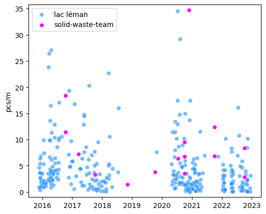
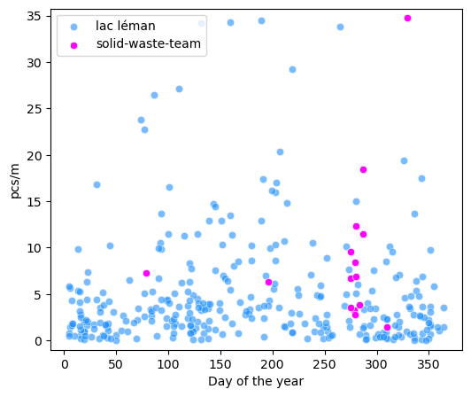
Lake Geneva sample totals

The total pcs/m for all surveys is given in figure 1 and figure 2. Samples after May 2021 are considered separately, this is a new six year sampling period for the lake. The distribution of the sample totals is given in table 2.

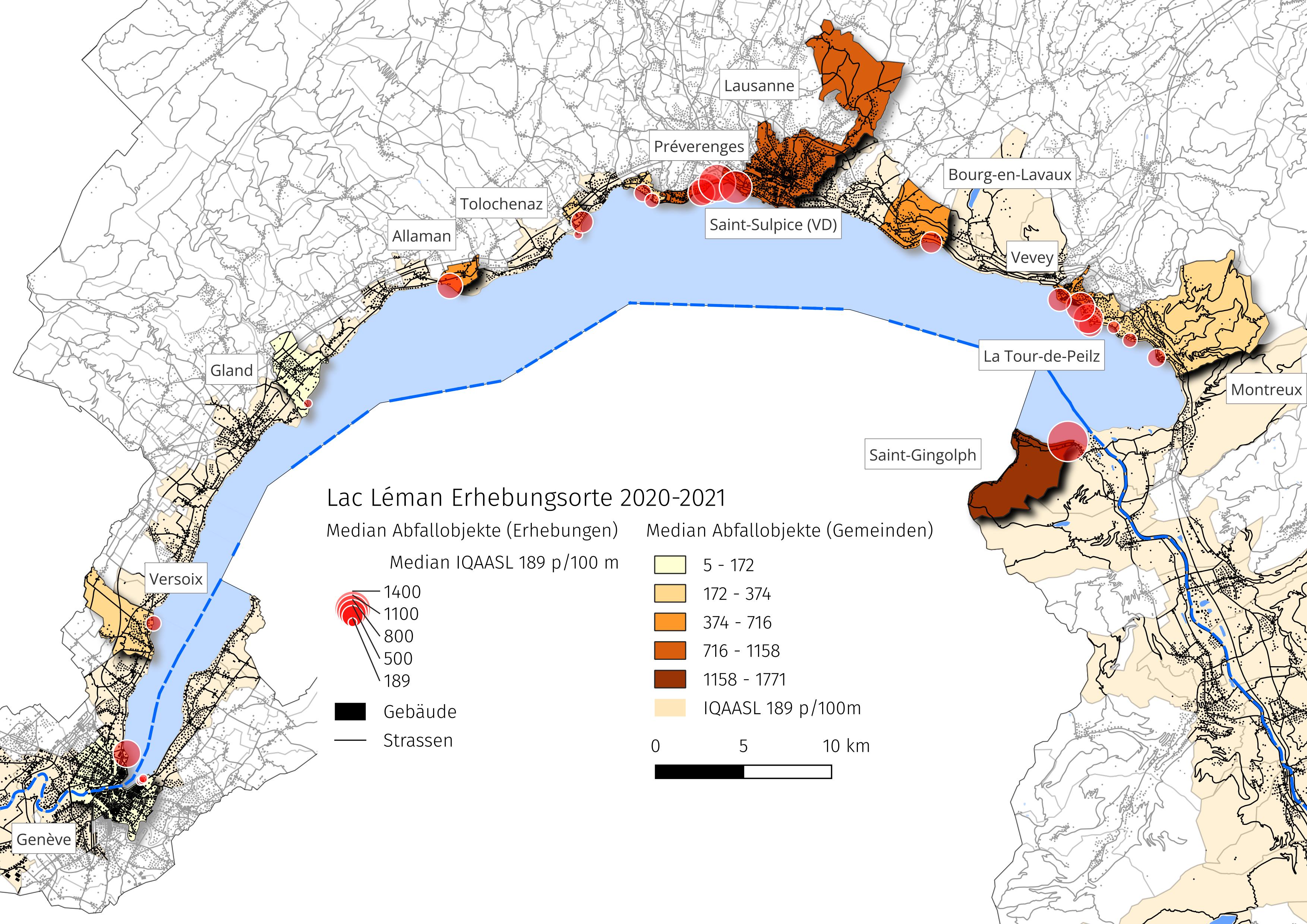
Fig. 3.1 Previous survey results from Lake Geneva

Figure 1, Table 2	Table 3, Figure 2
	The observed values from the training and testing data. Remark that the testing data is only 22% of all the data. This is because we are only in the first year of a six year sampling period   before may 2021 after may 2021 weight all samples 0.78 0.22 Number of samples 263 73 Median 3.47 2.28 Average 6.13 3.25 25th percentile 1.52 0.78 75th percentile 6.69 4.31
The number of different locations and cities for the data. Note that there are 31 different municipalitites in all.   before may 2021 after may 2021 Number of cities 21 19 Number of locations 48 23 Total objects 57,623 14,703

3.3. Expected survey results Saint Sulpice

3.3.1. Predicted values using empirical Bayes method

The method proposed in chapter two produced the following expected survey results for October 5, 2023 at Saint Sulpice:

Table 4: The 94% probability interval of the objects of interest for Saint Sulpice. The median value is used for the predictions

	G112	G27	G30	G32	G67	G70	G95	G96	Gcaps	Gfrags
3%	0.00	0.00	0.00	0.00	0.00	0.00	0.00	0.00	0.00	0.00
25%	0.00	0.05	0.03	0.00	0.05	0.00	0.01	0.00	0.04	0.00
48%	0.08	0.46	0.35	0.03	0.16	0.00	0.32	0.04	0.11	0.68
50%	0.12	0.47	0.39	0.04	0.16	0.01	0.32	0.04	0.11	0.74
52%	0.22	0.48	0.43	0.04	0.22	0.02	0.34	0.05	0.12	0.74
75%	0.68	0.93	0.57	0.08	0.33	0.05	0.52	0.08	0.23	1.24
97%	1.46	1.47	1.21	0.11	0.64	5.58	1.11	0.20	0.50	5.05

Recall that the previous results from Saint Sulpice are not used to make the predictions. Only locations in the same region with similar land-use characteristics are used.

3.3.2. Estimates from participants

After a classroom discusion and review of the previous years results (but not the predicted results) the participants made an estimate of how many they expect to find of each item of interest.

Table 5: The estimated amount in pcs/meter for each object that the participants expected to find.

	G112	G27	G30	G32	G67	G70	G95	G96	Gcaps	Gfrags
0	0.16	1.12	0.54	0.05	0.30	0.08	0.39	0.04	0.31	1.34
1	0.15	0.57	0.24	0.08	0.05	0.05	0.16	0.10	0.14	0.22
2	0.05	0.80	0.20	0.02	0.15	0.04	0.30	0.01	0.25	1.20
3	0.10	0.35	0.15	0.03	0.05	0.01	0.06	0.10	0.15	0.50
4	0.07	0.15	0.05	0.02	0.01	0.00	0.04	0.01	0.08	0.12
5	0.15	0.50	0.30	0.03	0.01	0.00	0.05	0.05	0.20	0.20
6	0.16	1.12	0.54	0.05	0.30	0.08	0.39	0.04	0.31	1.34
7	6.00	3.00	0.60	0.10	0.40	0.03	0.80	1.00	2.00	1.34
8	0.40	1.50	0.30	0.10	1.10	0.01	0.50	0.20	0.40	2.00

3.4. Survey results October 5, 2023 Saint Sulpice

After the particpants completed the forms, surveys were conducted at three beaches within the city limits of Saint Sulpice. Only the forms for two beaches were returned.

Table 6: The survey results of the objects of interest on October 5, 2023 in pieces per meter

	G112	G27	G30	G32	G67	G70	G95	G96	Gcaps	Gfrags
tiger-duck-beach	0.67	3.64	0.55	0.18	0.00	0.00	0.79	0.06	0.18	10.85
parc-des-pierrettes	0.08	1.03	0.14	0.04	0.00	0.00	0.24	0.02	0.24	5.40

3.5. Survey results October 5, 2023 Saint Sulpice

After the particpants completed the forms, surveys were conducted at three beaches within the city limits of Saint Sulpice. Only the forms for two beaches were returned.

Table 6: The survey results of the objects of interest on October 5, 2023 in pieces per meter

	G112	G27	G30	G32	G67	G70	G95	G96	Gcaps	Gfrags
tiger-duck-beach	0.67	3.64	0.55	0.18	0.00	0.00	0.79	0.06	0.18	10.85
parc-des-pierrettes	0.08	1.03	0.14	0.04	0.00	0.00	0.24	0.02	0.24	5.40

3.6. Results: Estimated, found and predicted

It appears that both the participants and the model underestimated the amount of plastic fragments. Recall that the participants were given the cumulative results for these objects, table 1.

Figure 3
Figure 3: The Estimated, observed and predicted results for the objects of interest, Saint Sulpice October 5, 2023

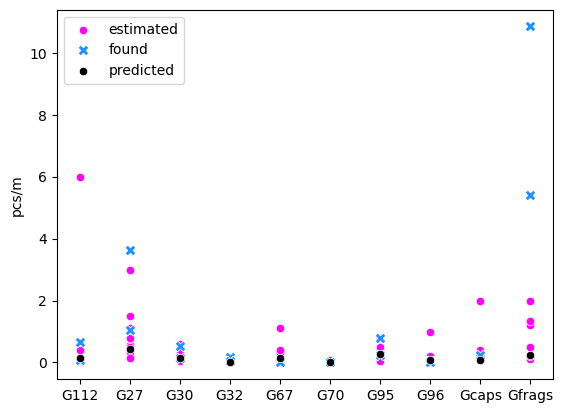
The predicted values from the model were all closer than the predicted values by the participants, table 7. In total 17/20 oserved results fell within the 96% probability interval predicted by the model, 7/20 fell within the 50% probability interval, Annex: table 8. Of the objects not within the 96% interval there is:

1. Fragmented plastics, (both surveys)

2. Cigarette ends

3. Toys and party favors

From figure 4 we can see how close the predictions and the estimates are.

Figure 4
Figure 4: The root of the squared difference between observed estimated and predicted, Saint Sulpice October 5, 2023

Table 7: The average difference between what was found and the estimates of the participants and what was predicted using the empirical Bayes method

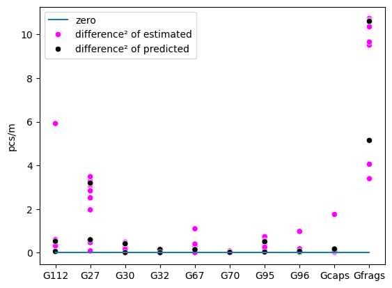
	average
source	difference² of estimated	difference² of predicted
G112	1.07	0.29
G27	2.32	1.87
G30	0.31	0.20
G32	0.11	0.07
G67	0.26	0.16
G70	0.03	0.01
G95	0.52	0.27
G96	0.15	0.02
Gcaps	0.26	0.10
Gfrags	8.11	7.38

3.7. Discussion

There were three surveys completed, two are reflected in the report. Neither the the estimated amounts from the particpants or the survey results were returned for the third survey. On location the participants were shown examples of the objects of interest. The limits of the survey area were defined and the survey was conducted in small groups. The objects found on the beach were separated and counted on location. The identification or the differentiation of fragmented plastics and foams remains difficult for new participants. This is in one part due to the constraints of time and on the other to the lack of experience. Many times what initially appears to be an unidentifiable piece of plastic can actually be placed in a more precise category with reasonable certainty. The new paritcipants do not have the time to consider other possibilities or simply are unaware of the original use of the item in questions.

Many participants used the previous aggregated survey results to estimate the expected values. This reasonable strategy produced estimates that were very close to the predicted survey results. This suggests that previous survey results can serve as an indicator for expected results as long as the objects have been identified correctly and consistently in the past. Yet, from table 7 it is clear that predictions are more accurate when a formal method is used.

3.8. Conclusions

From this experience we conclude that the expected values in table 4 do represent probable beach-litter densities in the region.

3.8.1. Next steps

Make hierarchical model

3.9. Annex

3.9.1. The accuracy of the predictions in relation to what was found

Table 8: Whether the observed value fell within the predicted interval

	object	within 96% HDI	within 50% HDI
0	G112	True	True
1	G27	False	False
2	G30	True	True
3	G32	False	False
4	G67	True	False
5	G70	True	False
6	G95	True	False
7	G96	True	True
8	Gcaps	True	True
9	Gfrags	False	False
0	G112	True	True
1	G27	True	False
2	G30	True	True
3	G32	True	True
4	G67	True	False
5	G70	True	False
6	G95	True	True
7	G96	True	True
8	Gcaps	True	False
9	Gfrags	False	False

within 96% HDI    0.80
within 50% HDI    0.45
dtype: float64

within 96% HDI    16
within 50% HDI     9
dtype: int64

This script updated 21/03/2024 in Biel, CH

❤️ what you do everyday: analyst at hammerdirt

Git repo: https://github.com/hammerdirt-analyst/solid-waste-team.git

Git branch: main

pandas    : 2.0.3
numpy     : 1.25.2
matplotlib: 3.7.1
seaborn   : 0.12.2